Secure machine learning against adversarial samples at test time

Abstract

Deep neural networks (DNNs) are widely used to handle many difficult tasks, such as image classification and malware detection, and achieve outstanding performance. However, recent studies on adversarial examples, which have maliciously undetectable perturbations added to their original samples that are indistinguishable by human eyes but mislead the machine learning approaches, show that machine learning models are vulnerable to security attacks. Though various adversarial retraining techniques have been developed in the past few years, none of them is scalable. In this paper, we propose a new iterative adversarial retraining approach to robustify the model and to reduce the effectiveness of adversarial inputs on DNN models. The proposed method retrains the model with both Gaussian noise augmentation and adversarial generation techniques for better generalization. Furthermore, the ensemble model is utilized during the testing phase in order to increase the robust test accuracy. The results from our extensive experiments demonstrate that the proposed approach increases the robustness of the DNN model against various adversarial attacks, specifically, fast gradient sign attack, Carlini and Wagner (C&W) attack, Projected Gradient Descent (PGD) attack, and DeepFool attack. To be precise, the robust classifier obtained by our proposed approach can maintain a performance accuracy of 99% on average on the standard test set. Moreover, we empirically evaluate the runtime of two of the most effective adversarial attacks, i.e., C&W attack and BIM attack, to find that the C&W attack can utilize GPU for faster adversarial example generation than the BIM attack can. For this reason, we further develop a parallel implementation of the proposed approach. This parallel implementation makes the proposed approach scalable for large datasets and complex models.

1 Introduction

Deep learning has been widely deployed in image classification [1–3], natural language processing [4–6], malware detection [7–9], self-driving cars [10, 11], robots [12], etc. For instance, the state-of-the-art performance of image classification on the ImageNet dataset increases from 73.8% (in 2011) to 98.7% (Top 5 Accuracy in 2020) utilizing deep learning models. This outstanding performance surpassed human annotators. However, in 2013, Szegedy et al. [13] showed the limitation of deep learning models, i.e., its inability to correctly classify the maliciously perturbed test instance that is apparently indistinguishable from its original test instance. Many other attacks, such as Fast Gradient Sign Method (FGSM) [14], DeepFool [15], and One-Pixel Attack [16], are introduced after Szegedy et al. [13] presented the Limited-memory Broyden Fletcher Goldfarb Shanno (L-BFGS) attack in 2013.

Adversarial examples are obtained by adding a small undetectable perturbation to original samples in order to mislead a DNN model to make a wrong classification. As shown in Fig. 1, Carlini and Wagner (C&W) attack [17] is applied to an image of number “5” from the MNIST dataset [18] to generate an image shown on the right in this figure. This generated image appears the same as the image on the left hand side. While the left image is classified as “5,” however, the right image is classified as “3” by a state-of-the-art digital recognition classifier whose performance accuracy is 99% on the MNIST test set. This result demonstrates the vulnerability of machine learning models.

Fig. 1

Two images, an arbitrary image of “5” from the cite reference [56] (left) and the corresponding adversarial example generated by the C &W’s attack (right), are indistinguishable to a human. However, the machine learning-based image recognition model (see Section 6.1 for neural network architectures) labels the left image as “5” and the right image as “3”

Various proactive and reactive defense methods against adversarial examples have been proposed over the years [19]. Examples of proactive defenses include adversarial retraining [14, 20], defensive distillation [21], and classifier robustifying [22, 23]. Examples of reactive defenses are adversarial detection [24–29], input reconstruction [30], and network verification [31, 32]. However, all defenses are later shown to be either ineffective for stronger adversarial attacks such as the C&W attack or cannot be applied to large networks. For instance, Reluplex [31] is only feasible for a network with only a few hundred neurons. In this work, we proposed a distributive retraining approach against adversarial examples that can preserve the performance accuracy even under strong attacks such as the C&W attack.

Contrary to some existing studies that attempt to detect the adversarial examples at the cost of reducing the classifier’s accuracy, we aim to maintain the classifier’s predicting accuracy by increasing model capacity and generating additional training data. Moreover, this proposed approach can be applied to any classifiers since it is classifier-independent. Particularly, the proposed approach is useful for safety- and security-critical systems, such as machine learning classifiers for malware detection [9] and autonomous vehicles [11].

Our proposed iterative approach can be considered as an adversarial (re)training technique. First, we train the model with normal images and normal images with random Gaussian noises added (the later ones are simply called noise images in this paper). Next, we generate adversarial images using attack techniques, such as PGD, DeepFool, and C&W attacks. Then, we retrain the model based on the adversarial images generated in the previous step, normal images, and noise images. This step can be considered as a combination of adversarial (re)training [13] and Gaussian data augmentation (GDA) [33]. However, we use soft labels instead of hard labels. Repeat this retraining process until the acceptable robustness or maximum iteration number is reached. The resulting classifier has n classes. The first n−1 classes are normal image classes, and the last one is the adversary class.

After the model is fully trained, we can test it. At the testing time, a small random Gaussian noise is added to a given test image before it is inputted into the model. Since our model is trained with Gaussian noise, it does not affect the classification of the normal images. However, if the test image is adversarial, it is likely to be generated from optimization algorithms that introduce well-designed minimal perturbation to a normal image. We can improve the likelihood of distinguishing the normal image from the adversarial image by disturbing this well-calculated perturbation with noises. Additionally, we propose an ensemble model in which a given test image without random noise is also input to the model, and its output is compared with the output of the test image with random noise added. If two outputs are the same, that is the final output of the model. If two outputs are different, a given test image is marked as adversarial to alert the system for further examination.

The key contributions of this paper are in the following:

• 1 We propose an iterative approach to training a model to either label the adversarial sample with the label of the original/natural sample or at least label it as the adversarial sample and alert the system for further examination. Compared to other studies, we treat the perturbation differently depending on its size. Our goal is to train a robust model that can classify the instance correctly when the perturbation η<η₀ and label it either correctly or as adversarial example when perturbation η≥η₀; that is, η is larger than some application specific perturbation limit η₀. This makes a better generalization as DNN models learn to focus on important features and ignore the unimportant ones.

• 2 The iterative process is highly parallelizable. Since the iterative model at time t is not much different from the iterative model at time t−1, the older model for generating adversarial examples should work as well as the current model due to the transferability of the adversarial examples. Some GPU nodes can be used to generate adversarial examples based on the previous iterative model instead of waiting for a new iterative model. Therefore, the adversarial example for the next iteration t can be generated before the new iterative model is produced.

• 3 The trained model based on our proposed methodology will not only be robust against adversarial examples but also maintains the accuracy of the original classifier. Some existing methods strengthen the model with respect to some attacks but reduce the accuracy of the classifier at the same time. Our model, through multiple data generating methods and larger network capacity, refines the data representation at each iteration; therefore, we can maintain our robustness and accuracy at the same time.

• 4 We proposed an ensemble model that outputs the final label based on the labels provided by two tests, one with added small random noise and one without. Small random noise is aimed to distort the optimal perturbation injected by the adversary. We have trained our model against random noise at training time; hence, the small random noise does not affect the classification accuracy of normal images. However, it may disturb the optimal adversarial example generated by an adversary. If the original image and image with added test noise produce different outputs from the model, the input image is likely to be adversarial.

The remainder of this paper is organized as follows. We introduce the threat model in Section 2. In Section 3, we present related work, and in Section 4, we provide the necessary background information. In Section 5, we present the proposed approach, followed by an evaluation in Section 6. In Section 8, we give conclusions and future work.

2 Threat model

Before discussing the related work, we define the threat model formally. In this work, we consider evasion attacks in both white-box settings (assume an adversary has full knowledge of the trained model F) and gray-box settings (assume an adversary has no knowledge of the trained model F but has knowledge of the training set used). The ultimate goal of an adversary is to generate adversarial examples x^′ that misled the trained model. That is, for each input (x,y), the adversary’s goal is to solve the following optimization problem:

$$\begin{array}{*{20}l} \operatorname*{min}_{\delta} \quad & ||\mathbf{x}-\mathbf{x}^{\prime}||_{2}^{2} \\ \textrm{s. t.} \quad & \mathbf{x}^{\prime} \in [0, 1]^{n}, F(\mathbf{x}^{\prime})=y^{\prime}, \end{array} $$

(1)

where y≠y^′ are class labels and ε is a maximum allowable perturbation that is undetectable by human eyes.

3 Related work

Over the past few years, various adversarial (re)training methods have been developed to mitigate adversarial attacks [14, 20]. Nevertheless, Tramèr et al. [34] showed that a two-step attack can easily bypass the classifier trained using adversarial examples by first adding a small noise to the system and then performing any classical attack technique such as FGSM and DeepFool. Instead of injecting adversarial examples to the training set, Zantedeschi et al. [35] suggested to add small noises to the normal images to generate additional training examples. They compared their methods with other defense methods, such as adversarial training and label smoothing, and showed that their approach is robust and does not compromise the performance of the original classifier. The last type of proactive countermeasures is to robustify a classifier. That is, its goal is to build more robust neural networks [22, 23]. For instance, in [22], Bradshaw combined DNN with Gaussian processes (GP) to make scalable GPDNN and showed that it is less susceptible to the FGSM attack.

Furthermore, Yuan et al. [19] introduced three reactive countermeasures for adversarial examples: adversarial detection [24–29], input reconstruction [30, 36], and network verification [31, 32]. Adversarial detection consists of many techniques for adversarial detecting. For instance, Feinman et al. [24] assumed that the distribution of adversarial sample is different from the distribution of natural sample and proposed a detection method based on the kernel density estimates in the subspace of the last hidden layer and the Bayesian neural network uncertainty estimates with dropout randomization. However, Carlini and Wagner [37] showed that the kernel density estimation, which is the most effective defense technique among ten defenses considered by Carlini and Wagner on MNIST, is completely ineffective on CIFAR-10. Grosse et al. [25] used Fisher’s permutation test with Maximum Mean Discrepancy (MMD) to check where a sample is adversarial or natural. Though MMD is a powerful statistical test, it fails to detect the C&W attack [37]. This indicates there may not be a significant difference between the distribution of an adversarial sample and the distribution of a natural sample when the adversarial perturbation is subtle. Xu et al. [29] used feature squeezing techniques to detect adversarial examples, and the proposed technique can be combined with other defenses such as the defensive distillation for defense against adversarial examples.

Input reconstruction is another category of reactive defense, where a model is used to find the distribution of a natural sample and an input is projected onto data manifold. In [30], a denoising contractive autodecoder network (CAE) is trained to transform an adversarial example to the corresponding natural one by removing the added perturbation. Song et al. [36] used PixelCNN, which provides the discrete probability of raw pixel values in the image, to calculate the probabilities of all training images. At the test time, a test instance is inputted and its probability is computed and ranked. Then, a permutation test is used to detect an adversarial perturbation. In addition, they proposed PixelDefend to purify an adversarial example by solving the following optimization problem:

$$ {\text{max}_{\mathbf{x}^{\prime}} P(\mathbf{x}^{\prime}) \text{ subject to} ||\mathbf{x}^{\prime}-\mathbf{x}||_{\infty} \leq \epsilon.} $$

(2)

Last but not the least, network verification formally proves whether a given property of a DNN model is violated. For instance, Reluplex [31] used a satisfiability modulo theory solver to verify whether there exists an adversarial example within a specified distance of some input for the DNN model with ReLU activation function. Later, Carlini et al. [38] showed that Reluplex can also support max-pooling by encoding max operators as follows:

$$ \text{max}(x,y)=ReLU(x-y)+y. $$

(3)

Initially, Reluplex could only handle the L_infty norm as a distance metric. Using Eq. (3), Carlini et al. [38] encoded the absolute value of sample x as

$$\begin{array}{*{20}l} |x| &= \text{max}(x,-x)=ReLU(x-(-x))+(-x) \end{array} $$

(4)

$$\begin{array}{*{20}l} &=ReLU(2x)-x. \end{array} $$

(5)

In this way, Reluplex can handle the L₁ norm as a distance metric as well. However, Reluplex is computationally infeasible for large networks. More specifically, it can only handle networks with a few hundred neurons [38]. Using Reluplex and k-means clustering, Gopinath et al. [32] proposed DeepSafe to provide safe regions of a DNN. On the other hand, Reluplex can be used by an attacker as well. For instance, Carlini et al. [38] proposed a Ground-Truth Attack that uses C&W attack as an initial step for a binary search to find an adversarial example with the smallest perturbation by invoking Reluplex iteratively. In addition, Carlini et al. [38] also proposed a defense evaluation using Reluplex to find a provably minimally distorted example. Since it is based on Reluplex, it is computationally expensive and only works on small networks. However, Yuan et al. [19] concluded that almost all defenses have limited effectiveness and are vulnerable to unseen attacks. For instance, C&W attack is effective for most of existing adversarial detection methods though it is computationally expensive [37]. In [37], authors showed that ten proposed detection methods cannot withstand white-box attack and/or black-box attack constructed by minimizing defense-specific loss functions.

4 Background

This section provides a brief introduction to neural networks and adversarial machine learning.

4.1 Neural networks

Machine learning automates the tasks of writing rules for a computer to follow. That is, giving an input and a desired outcome, machine learning can find a set of rules needed automatically. Deep learning is a branch of machine learning that automates a feature selection process. That is, you do not even need to specify the features, and a neural network can extract them from raw input data. For instance, in image classification, an image is inputted into the neural network and the convolutional layers of the neural network will extract the important features from the image directly. This makes deep learning desirable for many complex tasks such as natural language processing and image classification, where software engineers have difficulty writing rules for a computer to learn such tasks.

The performance of a neural network is remarkable in domains such as image classification [1–3], natural language processing [4–6], and machine translation [39]. By using the Universal Approximation Theorem [40], any continuous function in a compact space can be approximated by a feed-forward neural network with at least one hidden layer and suitable activation function to any desirable accuracy [41]. This theorem explains the wide application of deep neural networks. However, it does not give any constructive guideline on how to find such universal approximator. In 2017, Lu et al. [42] established the Universal Approximation Theorem for width-bounded ReLU networks, which showed that a fully connected width-(n+4) ReLU networks, where n is the input dimension, is an universal approximator. These two Universal Approximation Theorems explain the ability of deep neural network to learn.

A feed-forward neural network can be written as a function F:X→Y, where X is its input space or sample space and Y is its output space. If the task is classification, Y is the set of discrete classes. If the task is regression, Y is a subset of Rⁿ. For each sample, x∈X,F(x)=f_L(f_L−1(...(f₁(x)))), where f_i(x)=A(w_i∗x+b),A(.) is an activation function, such as the non-linear Rectified Linear Unit (ReLU), sigmoid, softmax, identity, and hyperbolic tangent (tanh); w_i is a matrix of weight parameters; b is the bias unit; i=1,2,…,L; and L is the total number of the layer in a neural network. For classification, the activation function for the last layers is usually a softmax function. The key to state-of-the-art performance of the neural network is the optimized weight parameters that minimize a loss function J, a measure of the difference between the predicted output and its true label. A common method used to find the optimized weights is the back-propagation algorithm. For example, see [43] and [44] for an overview of the back-propagation algorithm.

In this paper, we consider the DNN models for image classification. A gray scaled image x has h×w pixels, i.e., x∈R^hw, where each component x_i is normalized so that x_i∈[0,1]. Similarly, for a colored image x with a RGB channel, x∈R^3hw. In the following subsection, we will consider the attack approaches for generating adversarial image x^′ from the natural or original image x, where x can be either gray scaled or colored.

4.2 Attack approaches

Adversarial example/sample x^′ is a generated sample that is close to natural sample x to human eyes but misclassified by a DNN model [13]. That is, the modification is so subtle that a human observer does not even notice it, but a DNN model misclassifies it. Formally, an adversarial sample x^′ satisfies the conditions that

• $||\mathbf {x}-\mathbf {x}^{\prime }||_{2}^{2}< \epsilon$, where ε is the maximum allowable perturbation that is not noticeable by human eyes.

• x^′∈[0,1].

• F(x^′)=y^′,F(x)=y, and y≠y^′, where y and y^′ are class labels.

In general, there are two types of adversarial attacks for DNN models: untargeted and targeted. In an untargeted attack, an attacker does not have a specific target label in mind when trying to fool a DNN model. In contrast, an attacker tries to mislead a DNN model to classify an adversarial sample x^′ as a specific target label t in a targeted attack. In 2013, Szegedy et al. [13] first generated such an adversarial example using the Limited-memory Broyden Fletcher Goldfarb Shanno (L-BFGS) attack. Given a natural sample x and a target label t≠F(x), they used the L-BFGS method to find an adversarial sample x^′ that satisfies the following box-constrained optimization problem:

$$ \min c ||\mathbf{x}-\mathbf{x}^{\prime}||_{2}^{2}+J(\mathbf{x}^{\prime}, t), $$

(6)

$$\text{subject to }\mathbf{x}^{\prime} \in [0,1]^{m} \text{and }F(\mathbf{x}^{\prime})=t,$$

where c is a constant that can be found by linear searching, and m=hw if the image is gray scaled and m=3hw if the image is colored. Because of this computational intensive linear searching method for optimal c, the L-BFGS attack is time consuming and impractical. Over the course of the next few years, many other gradient-based attacks are proposed, for example,

• Fast Gradient Sign Method (FGSM)

  FGSM is a one-step algorithm that generates perturbations in the direction of the loss gradient, i.e., the amount of perturbation is

  $$ \eta = \epsilon \text{sgn}(\nabla_{x} J(x, l)) $$

  (7)

  and

  $$ \mathbf{x}^{\prime} = \mathbf{x} + \epsilon \text{sgn}(\nabla_{x} J(x, l)), $$

  (8)

  where ε is an application-specific imperceptible perturbation adversary intent to inject, and sgn(∇_xJ(x,l)) is the sign of the loss function [14]. The Basic Iterative Method (BIM) is an iterative application of FGSM in which a finer perturbation is obtained at each iteration. This method is introduced by Kurakin et al. [45] for generating an adversarial example in the physical world. The Projected Gradient Descent (PGD) is a popular variate of BIM that initializes through uniform random noise [46]. Iterative Least-likely Class Method (ILLC) [45] is similar to BIM but uses the least likely class as the targeted class to maximize the cross-entropy loss; hence, this is a targeted attack algorithm.

• Jacobian-based Saliency Map Attack (JSMA)

  JSMA uses the Jacobian matrix of a given image to find the input features of the image that made most significant changes to output [47]. Then, the value of this pixel is modified so that the likelihood of the target classification is higher. The process is repeated until the limited number of modifiable pixels is reached or the algorithm has succeeded in generating the adversarial example that is misclassified as a target class. Therefore, this is another targeted attack but has a high computation cost.

• DeepFool

  DeepFool searches for the shortest distance to cross the decision boundary using an iterative linear approximation of the classifier and orthogonal projection of the sample point onto it [15], as shown in Fig. 2. This untargeted attack generates adversarial examples with a smaller perturbation compared with L-BFGS, FGSM, and JSMA [17, 48]. For detail, see [15]. Universal Adversarial Perturbation is an updated version of DeepFool that is transferable [49]. It uses the DeepFool method to generate the minimal perturbation for each image and find the universal perturbation that satisfies the following two constraints:

  $$\begin{array}{@{}rcl@{}} && ||\eta||_{p} \leq \epsilon, \end{array} $$

  (9)

  Fig. 2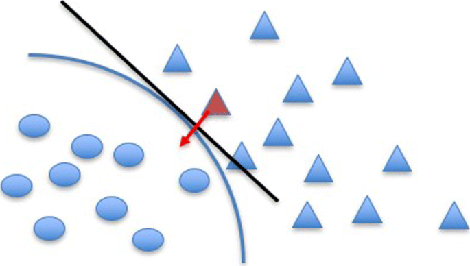

  

  DeepFool. The DeepFool attack approximates the decision boundary close to a targeted instance (triangle) by a linear line and searches for the shortest distance to cross the boundary and achieve targeted misclassification

  $$\begin{array}{@{}rcl@{}} && P(F(\mathbf{x}) \neq F(\mathbf{x}+\eta))> 1-\delta, \end{array} $$

  (10)

  where ||∗||_p is the p-norm, ε specifies the upper limit for perturbation, and δ∈[0,1] is a small constant that specifies the fooling rate of all the adversarial images.

• Carlini and Wagner (C&W) attack

  C&W attack [17] is introduced as a targeted attack against defensive distillation, a defense method against an adversarial example proposed by Papernot et al. [21]. Opposed to Eq. 6, Carlini and Wagner defined an objective function f such that f(x^′)≤0 if and only if F(x^′)=t, and the following optimization problem is solved to find the minimal perturbation η:

  $$\begin{array}{@{}rcl@{}} && \min ||\eta||_{2}^{2}+cf(\mathbf{x}^{\prime}), \end{array} $$

  (11)
  $$\begin{array}{@{}rcl@{}} && \text{ subject to }\mathbf{x}^{\prime} \in [0,1]^{m}. \end{array} $$

  (12)

  Instead of looking for optimal c using the linear searching method as in the L-BFGS attack, Carlini and Wagner observed that the best way to choose c is to use the smallest value of c for which f(x^′)≤0. To ensure that the box-constraint x^′∈[0,1]^m is satisfied, they proposed three methods, projected gradient descent, clipped gradient descent, and change of variable, to avoid box-constraint. These methods also allow us to use other optimization algorithms that do not naturally support box constraints. In their paper, the Adam optimizer is used since it converges faster than the standard gradient descent and the gradient descent with momentum. For detail, see [17]. C&W attack is not only effective for defensive distillation but also effective for most of existing adversarial detecting defenses. In [37], Carlini and Wagner used C&W’s attack against ten detection methods and showed the current limitations of detection methods. Though the C&W attack is very effective, it is computationally expensive compare to other techniques.

There are other attack techniques that assume a less powerful attacker who has no access to the model. These are called black-box attacks. Following are some of the black-box attack techniques proposed in past few years.

• Zeroth-order Optimization (ZOO)-based Attack estimates the gradient and Hessian using the quotient difference [50]. Though this eliminates the need for direct access to gradient, it requires a high computation cost.

• One-Pixel Attack uses differential evolution to find a pixel to modify. The success rate is 68.36% for CIFAR-10 test dataset and 16.04% for ImageNet dataset on average [16]. This shows the vulnerability of DNNs.

• Transfer attack generates adversarial samples for a substitution model and uses these generated adversarial samples to attack the targeted model [51]. This is often possible due to the transferability of DNN models.

• Natural GAN uses Wasserstein Generative Adversarial Networks (WGAN) to generate adversarial examples that look natural for tasks such as image classification, textual entailment, and machine translation [52]. Similarly, the Domain name GAN (DnGAN) [53] uses GAN to generate adversarial DGA examples and tests its performance on Bayes, J48, decision tree, and random forest classifier. Moreover, the authors [53] also used these generated adversarial examples along with normal training data to train a long short-term memory (LSTM) model and show a 2.4% increase in accuracy compared to the LSTM model trained with a normal training set alone. As another application, Chen et al. [54] use WGAN to denoise cell images.

5 Methodology

In this section, we present our iterative approach for generating more data from the original dataset to train our proposed model. The training process can be summarized in the following steps:

• 1 Generate adversarial examples using existing adversarial example crafting techniques. In the evaluation section, we only use the PGD and C&W attacks to generate adversarial examples since they are the two strongest attacks in existence and we have limited computation resource.

• 2 Generate more noisy images by adding the small random noises to the regular images. This is needed to make sure that the final model is not skewed toward the current methods for generating adversarial examples, and we want our final model to be robust against random noise.

• 3 Combine the regular training set with the adversarial images and noisy images generated in 1 and 2, respectively, to train the model. Instead of hard labels for these images, soft labels are used instead. For instance, hand-written “7” and “1” are similar in that both have a long vertical line. Hence, rather than label a hand-written digit as 100% “7” or 100% “1”. We may say it is 80% “7” and 20% “1”. This shows the structure similarity between “7” and “1”. More precisely, the soft labels for an adversarial image, a random image, and a clean image are defined as follows, respectively. Let τ be a hyperparameter that measures the acceptable size of perturbation. Let us first define the soft label, p_i(x_j), for an adversarial image based on the value of τ in the following two cases.

  • (a) If η<τ, then we define the soft label $p_{i}(x_{j})=\alpha +\frac {1-\alpha }{n}$ for the adversarial image $x^{\prime }_{j}$ generated using the real image x_j that belongs to class i, and $\frac {1-\alpha }{n}$ otherwise, where 0<α<1 is close to 1 and n is the number of classes.

  • (b) If η≥τ, we define the soft label p_i(x_j)=β for the adversarial image $x^{\prime }_{j}$ generated using the real image x_j that belongs to class i, the soft label p_n(x_j)=γ for the adversarial image $x^{\prime }_{j}$ generated using the real image x_j that belongs to the adversarial class, and the soft label $p_{k}(x_{j})=\frac {1-\beta -\gamma }{n-2}$ for adversarial image $x^{\prime }_{j}$ generated using the real image x_j that belongs to class k, where k≠i,n,0<β,γ<1, and 0<β+γ<1.

  The soft label for a random-noise image is defined similarly. The α and τ values used for soft label calculation of adversarial images and random noise images are shown in Table 1. For simplicity, the correct class is assigned a soft label of 0.95, whereas other classes are assigned a soft label of 0.05/9 for the clean images.

  Table 1 Training parameters

• 4 Check robustness of the model if it is used as a stopping criterion. In [35], the robustness of a model is defined in terms of the expected amount of L₂ perturbation that is required to fool the classifier:

  $$ \rho=E_{(x,y)} \frac{\eta}{||x||_{2}+\delta}, $$

  (13)

  where η is the amount of L₂ perturbation that an adversary added a perturbation to a normal image x, and δ is an extremely small constant allowing for the division to be defined, say δ=10⁻¹⁰. We use this definition of robustness in this paper since this definition captures the intuition that larger perturbation is required to fool the classifier indicates a more robust classifier.

• 5 While k<k_max and/or the robustness of the model ρ<ρ₀, where ρ₀ is an acceptable level of robustness selected by an user and k_max is the maximum number of iterations allowed, this step repeatedly generates and accumulates a large amount of data for training a robust model.

  • (a) Sample a mini-batch of N stratified random images from a real image set and generate additional images using adversarial example generating techniques (shown in step 1) and random perturbation (shown in step 2). This combined sample is then used in the next step to retrain the model.

  • (b) Retrain the model. Update the model weights by minimizing the following cross-entropy loss:

    $$ J_{D}=-\frac{1}{N}\sum_{j=1}^{N} \sum_{i=1}^{n} p_{i}(x_{j}) \log (q_{i}(x'_{j})), $$

    (14)

    where n is the number of classes. The n^th class is the adversarial class, whereas classes 1 to n−1 are regular image classes.

The implications of the above proposed approach are discussed in Section 7, where we have showed that our proposed approach is robust when a small noise is injected to the test instance before the classification is performed, and it is also robust against both white-box attacks and black-box attacks. However, we have not studied whether or not our proposed approach is robust against adaptive attacks. A further study is needed in the future.

6 Evaluation

In this section, we empirically evaluate our proposed approach on MNIST [18] dataset and CIFAR-10 [55], canonical datasets used by most papers for attack and defense evaluation [21, 29]. The performance metric considered is the accuracy of the classifier.

6.1 Datasets

The MNIST handwritten digit recognition dataset [56] is a subset of a larger set available from NIST. It is normalized, where each pixel is ranged between 0 and 1 and each image has 28×28 pixels. There are 10 classes: the digits 0 through 9. All the images are black and white. The samples are split between a training set of 60,000 and a test set of 10,000. Out of 60,000 training instances, 10,000 are reserved for validation, and 50,000 are used for actual training. To evaluate the scalability of the proposed robust classifier, we consider CIFAR-10, which is a 32×32×3 colored image dataset consisting of 10 classes: airplane, automobile, bird, cat, deer, dog, frog, horse, ship, and truck. The samples are split between a training set of 50,000 and a test set of 10,000. See Table 2 for a summary of the dataset parameters.

Table 2 Dataset summary

6.2 Network architectures

The network architecture for the MNIST dataset consists of two ReLU convolutional layers, one with 32 filters of size 3 by 3 and follows by another with 64 filters of size 3 by 3. Then, a 2 by 2 max-pooling layer and a dropout with a rate of 0.25 is applied before a ReLU fully connected layer with 1024 units. The last layer is another fully connected layer with 11 units and a softmax activation function for classification in 10 regular classes plus an adversarial class. The total number of the parameters is 6,616,970 for the original model with 10 regular classes only. The proposed model with 11 classes has 6,617,995 parameters. The accuracy of the model is 99%, which is comparable to the accuracy of the state-of-the-art DNN. The network architecture for the CIFAR-10 model is a ResNet-based model provided by the IBM [57]. The hyperparameters used for the training and the corresponding values are shown in the following table. For instance, we set the acceptable level of robustness ρ₀ to 0.1.

6.3 Adversarial crafting

We use Adversarial Robustness Toolbox (ART v0.10.0) [57] to generate adversarial examples for training and test. The training set is used to generate the adversarial examples for training, and the test set is used to generate the adversarial examples for test. Due to the limited computing resource, we only use BIM and C&W attacks and Gaussian noise to generate additional images for training. The BIM and C&W attacks are selected over others because they generate the strongest attacks [46], and Gaussian noise is added to the images to take care of other potential attacks and for better data representation. The soft labels for those images are based on the perturbation introduced. For instance, under the C&W attack, we use a soft label of 0.44 if the perturbation limit is less than 0.026. 0.026 is selected based on the observation that the perturbation within this limit is hardly noticeable to human eyes. For a similar reason, the perturbation limit of BIM and Gaussian noise is set to 0.15 and 0.25 with a soft label value of 0.44.

At the test time, we consider the strong white-box attack against our proposed model. The adversarial images are generated using FGSM, DeepFool, and C&W attack with the assumption that an adversary has feature knowledge, algorithm knowledge, and the ability to inject adversarial images. FGSM attack is selected because it is a popular attack technique using by many papers for evaluation. BIM, DeepFool, and C&W attacks are selected because they are the three currently strongest existing attacks. For the FGSM attack, the perturbation of ε=0.1 is considered. This is a reasonable limit because a larger perturbation can be detected by human and/or anomaly detection systems. Similarly, the maximum perturbation for the BIM attack is also set to 0.1 and the attack step size is set to $\frac {0.1}{3}$. The maximum number of iterations for BIM is 40. The settings of the C&W and DeepFool attacks are left as default in ART [57]. Random noise added to train images follows a Gaussian distribution with mean 0 and variance η_max for each batch.

6.4 Results

We consider the accuracies of the classifiers on the normal MNIST and CIFAR-10 test images and the accuracies of the classifier under FGSM, C&W, BIM, and DeepFool attacks, respectively. The prediction accuracy of the original classifier on the normal MNIST test images is 99%. The prediction accuracy of the robust classifier on the normal MNIST test images is also 99% after retraining. Furthermore, the accuracies of the robust classifier under FGSM, C&W, BIM, and DeepFool attacks are shown in Table 3. These results have shown that after retraining, the model performance dramatically improved under these attacks. As shown, the original model’s classification accuracy drops significantly under the attacks. On the contrary, our robust classifier maintains the classification accuracy even under the attacks. Compared to the adversarial retraining method implemented by IBM’s adversarial robustness toolbox, our robust classifier performs better under DeepFool and C&W attacks.

Table 3 Classification accuracy on the MNIST test dataset under the white-box attack

To evaluate the performance of the classifiers under gray-box attacks, we assume that an attacker has no knowledge of a neural architecture. In this case, an attacker builds his/her own approximated CNN model and conducts the transfer attacks. We assume that an attacker develops a simple CNN model consisting a CNN layer with 4 filters of size 5 by 5, followed by a 2 by 2 max-pooling layer and a fully connected layer with 10 units and a softmax activation function for classification. The accuracy of the model is 99%, which is comparable to the accuracy of the state-of-the-art [48]. Table 4 shows that the original model performs poorly under grey-box attack. In fact, it is worsen than what is under the white-box attack. However, the black-box attacks have little affected under the adversarially retrained models.

Table 4 Classification accuracy on the MNIST test dataset under the gray-box attack

Moreover, a similar experiment has been performed on the CIFAR-10 dataset for the evaluation of the scalability of the proposed robust classifier. The experimental results are shown in Table 5. Note that we do not conduct any hyperparameter tuning due to the constraints of HPC cluster resource and time. That is, we have used the same hyperparameter settings, as shown in Table 1. The robust classifier performs better than the original model, though the improvement is not as good as for the MNIST dataset. As shown in this table, the accuracy has been improved by 31%, 32%, 72%, and 23% under FGSM, CW, BIM, and Deep Fool attack, respectively.

Table 5 Classification accuracy on the CIFAR-10 test dataset under white-box attacks

7 Discussion

In this section, the implications of the mechanism are discussed.

7.1 Trade-off between the accuracy and resilience against adversarial examples

One common problem of adversarial training and other defense methods is the trade-off between the accuracy and resilience against adversarial examples. This trade-off exists because the network architectures of an original system and its proposed one are similar and/or the dataset size is fixed. However, our proposed approach has a larger network capacity with a larger dataset generated by multiple techniques. Hence, our proposed approach does not have this trade-off as shown in Section 6. This solves the problem of trade-off between the accuracy and the robustness against an adversarial example and makes the model not only robust against a strong adversarial attack but also maintains the performance for classification. See Section 6 for detail.

7.2 Training time

Another consideration is the training time. To check the number of epochs needed for the training, the model is trained for ten epochs, as shown in Fig. 3. The total training time for ten epochs is about 90 s on Google Colab (with 12GB NVIDIA Tesla K80 GPU). To prevent overfitting, three epochs are selected for training the original model. A similar procedure is used to determine that ten epochs are needed for the proposed model. However, the proposed approach is highly parallelizable. Due to the transferability of adversarial examples, the adversarial examples do not have to be generated using the current model. Hence, adversarial crafting and adversarial training can be performed simultaneously. That is, at iteration t, an adversarial example can be generated based on the model generated at iteration t^′<t, and adversarial training can be performed using the adversarial example generated previously as well. Depending on the memory and computation resource, we can store the generated adversarial example at each iteration and sample from it when performing the adversarial training. The sampling probability can be based on the performance of the model at previous iterations. For instance, initially, we assign a probability of $\frac {1}{n}$ to each adversarial example and increases its probability for the next iteration if the model misclassifies it or it is not selected for the current iteration of training and decreases its probability if the model correctly classifies it. Furthermore, we can parallelize the adversarial crafting step (or the fake image generation step) by assigning a CPU (or GPU) for each adversarial crafting technique. Similarly, data parallelization can be performed during training.

Fig. 3

Training and validation loss. The training loss decreases with every epoch, whereas the validation loss does not decrease much after the third epoch. Hence, the training process can be stopped after three epochs to prevent overfitting

The framework for parallelization is shown in Fig. 4. Initially, the original model and a random sample of the original images are used to generate fake images. The original model is needed because we want to generate adversarial images by just adding an application-specific imperceptible perturbation to the original image and make it misclassified by the original model. There are various ways to obtain such an application-specific imperceptible perturbation. For instance, the FGSM attack generates such a perturbation by using the model’s loss gradient as described in Section 4. After the fake images are generated, it is saved to the fake image storage folder. During the retraining step, a random sample of fake images and original images as well as the copies of the original model are sent to the multiple-GPUs for retraining. After the retraining, the updated model is checked to see if it is robust against adversarial attacks. If so, the updated model is saved, and the process ends. Otherwise, the updated model is saved as the new model for the next stage of fake image generation and retraining.

Fig. 4

Parallelization framework. We decouple the fake image generation step from the retraining step by only updating the model used for the fake image generation as a new model is obtained. This way, the fake image generation step can continuously generate adversarial images while the retraining continues. Furthermore, the fake image generation step is parallelized by using multi-processing. Note that the processors can be GPUs or CPUs. GPUs are better in term of computation efficiency, and CPUs can store more images

To demonstrate the importance of selecting right the resource for different adversarial example crafting techniques, we conduct an experiment on a standard alone personal computer (12 thread CPUs). First, we independently run each attack on the same computer and measure the run time for generating a batch of 64, 128, 256, and 512 adversarial examples without GPU resource. To reduce the variation, we repeat the same experiment for 30 times for each attack. Then, we install K40C, TitanV, and both K40C and TitanV, respectively, and repeat the experiments. The result is shown in Figs. 5 and 6. The BIM attack run faster on CPU than on GPUs. In fact, when an attacker tries to utilize the GPUs, the adversarial image generation speed goes down. As shown in Fig. 5, though we utilize different types of GPU, the adversarial image generation speed does not change among the GPU types. On the contrary, C&W attack takes advantage of the GPU and runs faster on GPU than on CPU. Furthermore, we see that C&W attack runs faster on Titan V than on K40c. Table 6 is obtained by averaging over batch sizes. As shown, the BIM attack runs twice as fast on CPU than GPU whereas C&W attack runs faster on GPU. The variation among the runs is smaller under BIM attacks on average, as shown with smaller standard deviations. Moreover, we create a row called Titan V + K40c (average), which takes the average speed of Titan V and K40c. Comparing the values on this row with the value in the last row, we see that actual speed with two GPUs is not equal to the average speeds if GPU is utilized (as in C&W attack).

Fig. 5

Adversarial image generation speed under the BIM attack. Image generation speeds under the BIM attack. Note that CPU has a much faster adversarial image generation speed than K40C, TitanV, and both K40C and TitanV

Fig. 6

Adversarial image generation speed under the C&W attack. Note that CPU has a much slower adversarial image generation speed than K40C, TitanV, and both K40C and TitanV in the attack. That is, the C&W attack has an opposite result than the BIM attack

Table 6 GPUs vs. CPU

7.3 Ensembling

At the test time, a small random noise is injected to the test instance before performing the classification. This small noise is aimed to distort the intentional perturbation injected by the adversarial. An experiment is performed to illustrate it as follows. First, 100 adversarial images are generated using two popular adversarial attack algorithms, BIM and FGSM. Then, using NumPy’s [58] normal number generator with a mean of 0.01 and variance of 0.01, a small random normal noise is generated for each adversarial image. This small random normal noise is injected into an adversarial image. Next, the original classifier classifies these noisy adversarial images. If the predicted label is different from the ground truth, then the attack is successful (we considered an untargeted attack). Otherwise, it is unsuccessful. This process is repeated 30 times. The average result is shown in Fig. 7. Even without robust adversarial training, the classifier (original) can reduce the attack success rate by 14% for the FGSM attack and 20% for the BIM attack when the perturbation injected by an attacker is 0.01. Even when the perturbation increases to 0.05, the injected random noise can reduce the attack success rate of FGSM and BIM by 6% and 14%, respectively.

Fig. 7

Reduction in the attack success rate (%) as a function of perturbation injected by the FGSM and BIM attacks, respectively

Since our proposed model is trained with random noise, it is robust against it. The small noise added to the natural image is not likely to change the label of the image since we have trained our model with small Gaussian noise. However, if the test instance is adversarial, then it is likely produced by an optimization algorithm that searches for a minimal perturbation to a clean image. However, the injected random noise to such a clean image will mess up such well-calculated minimal perturbation. Therefore, if the label of a given test image without added random noise is different from that of with added random noise, this is likely an adversarial image and the system is alerted.

7.4 Limitations

Section 6 considered both white-box attacks (the attacker knows model architecture) and black-box attacks (the attacker does not know the model architecture). The proposed model is robust against both types of attacks, as shown in Section 5. However, those evaluations are based on the MNIST dataset. More experimentation on larger datasets are encouraged if the computational resource is available. Furthermore, it is unclear whether or not our proposed approach is still robust when crafting adversarial samples are done by someone who has no idea what toolboxes like ART are used. We will answer this question in our further studies.

In Section 6.2, we discussed the training time and proposed a parallelization framework for adversarial training. Then, to show the importance of selecting the right resource, we experimented on different types of GPUs. In Section 6.3, we discussed the idea of ensembling and performed an experiment to show the effectiveness of random noise in reducing the attack success rate on the original model (without adversarial training) under FGSM and BIM attacks. Note that all attacks are generated based on the Adversarial Robustness Toolbox. However, similar results can be obtained using other toolboxes such as Foolbox [59] or advertorch [60]. Furthermore, it is encouraged to test the proposed defense method on a tailored adaptive attack that might generate successful perturbations on randomly perturbed images instead of clean images.

8 Conclusions and future work

Many recent researchers have utilized various machine learning techniques, such as DNN, for security-critical applications. For instance, Morgulis et al. [61] have demonstrated that traffic sign recognition systems of a car can be easily fooled by adversarial traffic signs and cause the car to take unwanted actions. This result has shown the vulnerability of machine learning techniques. In this work, we have presented a distributed adversarial retraining approach against adversarial examples. The proposed methodology is based on the idea that with enough datasets, sufficient complex neural network, and computational resource, we can obtain a DNN model that is robust against these adversarial attacks. The proposed approach is different from the existing adversarial retraining approach in several aspects. First, we have used soft label instead of hard label to prevent overfitting. Second, we have proposed to increase model complexity to overcome the trade-off between the model accuracy and the resilience against adversarial examples. Furthermore, we have utilized the transferability property of adversarial instance to develop a distributive adversarial retraining framework that can save runtime when multiple GPUs are available. In addition, we have robustly trained the DNN model against random noise. Therefore, the obtained final classifier can provide the correct labeling to a normal instance, even though that the instance has random Gaussian noise added. By utilizing this robustness against random noise, we have added random noise to all test instances before performing classification in order to break the careful calculated adversarial perturbation. Moreover, we have compared our proposed approach against the current start-of-the-art approach and demonstrated that our proposed approach can effectively defend against stronger adversarial attacks, i.e., C&W attack and Deepfool. Future work will explore black-box attacks and formal guarantee for performance.

References

E. Real, A. Aggarwal, Y. Huang, Q. V. Le, Regularized Evolution for Image Classifier Architecture Search. Proc. AAAI Conf. Artif. Intell. 33(01), 4780–4789 (2019). https://doi.org/10.1609/aaai.v33i01.33014780.
B. Zoph, V. Vasudevan, J. Shlens, Q. V. Le, in Proceedings of the IEEE Conference on Computer Vision and Pattern Recognition. Learning transferable architectures for scalable image recognition, (2018), pp. 8697–8710.
J. Hu, L. Shen, G. Sun, in Proceedings of the IEEE Conference on Computer Vision and Pattern Recognition. Squeeze-and-excitation networks, (2018), pp. 7132–7141.
C. -C. Chiu, T. N. Sainath, Y. Wu, R. Prabhavalkar, P. Nguyen, Z. Chen, A. Kannan, R. J. Weiss, K. Rao, E. Gonina, et al, in 2018 IEEE International Conference on Acoustics, Speech and Signal Processing (ICASSP). State-of-the-art speech recognition with sequence-to-sequence models (IEEECalgary, 2018), pp. 4774–4778.
J. Devlin, M. -W. Chang, K. Lee, K. Toutanova, in Proceedings of the 2019 Conference of the North American Chapter of the Association for Computational Linguistics: Human Language Technologies, NAACL-HLT 2019, Minneapolis, MN, USA, June 2-7, 2019, Volume 1 (Long and Short Papers), ed. by J. Burstein, C. Doran, and T. Solorio. BERT: Pre-training of Deep Bidirectional Transformers for Language Understanding (Association for Computational Linguistics, 2019), pp. 4171–4186https://doi.org/10.18653/v1/n19-1423.
G. Hinton, L. Deng, D. Yu, G. Dahl, A. -R. Mohamed, N. Jaitly, A. Senior, V. Vanhoucke, P. Nguyen, B. Kingsbury, et al, Deep neural networks for acoustic modeling in speech recognition. IEEE Signal Process. Mag.29:, 82–97 (2012).
W. Xu, Y. Qi, D. Evans, in 23rd Annual Network and Distributed System Security Symposium, NDSS 2016, San Diego, California, USA, February 21-24, 2016. Automatically Evading Classifiers: A Case Study on PDF Malware Classifiers (The Internet Society, 2016). http://wp.internetsociety.org/ndss/wp-content/uploads/sites/25/2017/09/automatically-evading-classifiers.pdf.
C. Nachenberg, J. Wilhelm, A. Wright, C. Faloutsos, in ACM KDD. Polonium: Tera-scale graph mining for malware detection (Washington, DC, 2010).
M. A. Rajab, L. Ballard, N. Lutz, P. Mavrommatis, N. Provos, in Network and Distributed Systems Security Symposium (NDSS). CAMP: Content-Agnostic Malware Protection (USA, 2013). http://cs.jhu.edu/~moheeb/aburajab-ndss-13.pdf.
J. H. Metzen, M. C. Kumar, T. Brox, V. Fischer, in 2017 IEEE International Conference on Computer Vision (ICCV). Universal adversarial perturbations against semantic image segmentation, (2017), pp. 2774–2783. https://doi.org/10.1109/ICCV.2017.300.
M Bojarski, D Del Testa, D Dworakowski, B Firner, B Flepp, P Goyal, LD Jackel, M Monfort, U Muller, J Zhang, X Zhang, J Zhao, K Zieba, End to End Learning for Self-Driving Cars. CoRR. abs/1604.07316: (2016). http://arxiv.org/abs/1604.07316.
V. Mnih, K. Kavukcuoglu, D. Silver, A. A. Rusu, J. Veness, M. G. Bellemare, A. Graves, M. Riedmiller, A. K. Fidjeland, G. Ostrovski, et al, Human-level control through deep reinforcement learning. Nature. 518(7540), 529 (2015).
C. Szegedy, W. Zaremba, I. Sutskever, J. Bruna, D. Erhan, I. J. Goodfellow, R. Fergus, in International Conference on Learning Representations (ICLR). Intriguing properties of neural networks, (2014).
I. J. Goodfellow, J. Shlens, C. Szegedy, in International Conference on Learning Representations. Explaining and harnessing adversarial examples, (2015).
S. -M. Moosavi-Dezfooli, A. Fawzi, P. Frossard, in Proceedings of the IEEE Conference on Computer Vision and Pattern Recognition. Deepfool: a simple and accurate method to fool deep neural networks, (2016), pp. 2574–2582.
J. Su, D. V. Vargas, K. Sakurai, One pixel attack for fooling deep neural networks. IEEE Trans. Evol. Comput.23:, 828–841 (2019).
N. Carlini, D. Wagner, in 2017 IEEE Symposium on Security and Privacy (SP). Towards evaluating the robustness of neural networks (IEEESan Jose, 2017), pp. 39–57.
Y. LeCun, L. Bottou, Y. Bengio, P. Haffner, et al, Gradient-based learning applied to document recognition. Proc. IEEE. 86(11), 2278–2324 (1998).
X. Yuan, P. He, Q. Zhu, X. Li, Adversarial examples: attacks and defenses for deep learning. IEEE Trans. Neural Netw. Learn. Syst.30:, 2805–2824 (2019). https://doi.org/10.1109/TNNLS.2018.2886017.
R Huang, B Xu, D Schuurmans, C Szepesvári, Learning with a Strong Adversary. CoRR. abs/1511.03034: (2015). http://arxiv.org/abs/1511.03034.
N. Papernot, P. McDaniel, X. Wu, S. Jha, A. Swami, in 2016 IEEE Symposium on Security and Privacy (SP). Distillation as a defense to adversarial perturbations against deep neural networks (IEEESan Jose, 2016), pp. 582–597.
J. Bradshaw, A. G. G. Matthews, Z. Ghahramani, Adversarial examples, uncertainty, and transfer testing robustness in Gaussian process hybrid deep networks. arXiv preprint arXiv:1707.02476. 108: (2017).
M Abbasi, C Gagné, Robustness to Adversarial Examples through an Ensemble of Specialists. CoRR. abs/1702.06856: (2017). http://arxiv.org/abs/1702.06856.
R Feinman, RR Curtin, S Shintre, AB Gardner, Detecting Adversarial Samples from Artifacts. CoRR. abs/1703.00410: (2017). http://arxiv.org/abs/1703.00410.
K Grosse, P Manoharan, N Papernot, M Backes, PD McDaniel, On the (Statistical) Detection of Adversarial Examples. CoRR. abs/1702.06280: (2017). http://arxiv.org/abs/1702.06280.
D Hendrycks, K Gimpel, in 5th International Conference on Learning Representations, ICLR 2017, Toulon, France, April 24-26, 2017, Workshop Track Proceedings. Early Methods for Detecting Adversarial Images (OpenReview.net, 2017). https://openreview.net/forum?id=B1dexpDug.
A. N. Bhagoji, D. Cullina, P. Mittal, Dimensionality Reduction as a Defense against Evasion Attacks on Machine Learning Classifiers. CoRR. abs/1704.02654: (2017). http://arxiv.org/abs/1704.02654.
X. Li, F. Li, in Proceedings of the IEEE International Conference on Computer Vision. Adversarial examples detection in deep networks with convolutional filter statistics, (2017), pp. 5764–5772.
W. Xu, D. Evans, Y. Qi, in 25th Annual Network and Distributed System Security Symposium, NDSS 2018, San Diego, California, USA, February 18-21, 2018. Feature Squeezing: Detecting Adversarial Examples in Deep Neural Networks (The Internet Society, 2018). http://wp.internetsociety.org/ndss/wp-content/uploads/sites/25/2018/02/ndss2018_03A-4_Xu_paper.pdf.
S. Gu, L. Rigazio, in 3rd International Conference on Learning Representations, ICLR 2015, San Diego, CA, USA, May 7-9, 2015, Workshop Track Proceedings, ed. by Y. Bengio, Y. LeCun. Towards Deep Neural Network Architectures Robust to Adversarial Examples, (2015). http://arxiv.org/abs/1412.5068.
G. Katz, C. Barrett, D. L. Dill, K. Julian, M. J. Kochenderfer, in International Conference on Computer Aided Verification, ed. by R. Majumdar, V. Kuncak. Reluplex: an efficient SMT solver for verifying deep neural networks (Springer, 2017), pp. 97–117.
D. Gopinath, G. Katz, C. S. Păsăreanu, C. Barrett, in Proceedings of the 16th International Symposium on Automated Technology for Verification and Analysis (ATVA ’18). Lecture Notes in Computer Science, vol. 11138, ed. by S. Lahiri, C. Wang. DeepSafe: A Data-driven Approach for Assessing Robustness of Neural Networks (SpringerLos Angeles, 2018), pp. 3–19. https://doi.org/10.1007/978-3-030-01090-4_1.
V. Zantedeschi, M. -I. Nicolae, A. Rawat, in Proceedings of the 10th ACM Workshop on Artificial Intelligence and Security. Efficient defenses against adversarial attacks (ACM, 2017), pp. 39–49.
F. Tramèr, A. Kurakin, N. Papernot, I. Goodfellow, D. Boneh, P. McDaniel, in 6th International Conference on Learning Representations, ICLR 2018, Vancouver, BC, Canada, April 30 - May 3, 2018, Conference Track Proceedings. Ensemble Adversarial Training: Attacks and Defenses (OpenReview.net, 2018). https://openreview.net/forum?id=rkZvSe-RZ.
V. Zantedeschi, M. -I. Nicolae, A. Rawat, in Proceedings of the 10th ACM Workshop on Artificial Intelligence and Security, AISec@CCS 2017, Dallas, TX, USA, November 3, 2017, ed. by B. M. Thuraisingham, B. Biggio, D. M. Freeman, B. Miller, and A. Sinha. Efficient defenses against adversarial attacks (ACM, 2017), pp. 39–49. https://doi.org/10.1145/3128572.3140449.
Y. Song, T. Kim, S. Nowozin, S. Ermon, N. Kushman, in 6th International Conference on Learning Representations, ICLR 2018, Vancouver, BC, Canada, April 30 - May 3, 2018, Conference Track Proceedings. PixelDefend: Leveraging Generative Models to Understand and Defend against Adversarial Examples (OpenReview.net, 2018). https://openreview.net/forum?id=rJUYGxbCW.
N. Carlini, D. Wagner, in Proceedings of the 10th ACM Workshop on Artificial Intelligence and Security. Adversarial examples are not easily detected: bypassing ten detection methods (ACMDallas, 2017), pp. 3–14.
N Carlini, G Katz, C. W. Barrett, D. L. Dill, Ground-Truth Adversarial Examples. CoRR. abs/1709.10207: (2017). http://arxiv.org/abs/1709.10207.
P. L. Garvin, On Machine Translation: Selected Papers, vol. 128 (Walter de Gruyter GmbH & Co KG, Netherlands, 2019).
K. Hornik, M. Stinchcombe, H. White, Multilayer feedforward networks are universal approximators. Neural Netw.2(5), 359–366 (1989).
A. R. Barron, Approximation and estimation bounds for artificial neural networks. Mach. Learn.14(1), 115–133 (1994).
Z. Lu, H. Pu, F. Wang, Z. Hu, L. Wang, in Advances in Neural Information Processing Systems. The expressive power of neural networks: a view from the width, (2017), pp. 6231–6239.
I. Goodfellow, Y. Bengio, A. Courville, Deep Learning (MIT press, Cambridge, MA, 2016). http://www.deeplearningbook.org.
J. Bergstra, F. Bastien, O. Breuleux, P. Lamblin, R. Pascanu, O. Delalleau, G. Desjardins, D. Warde-Farley, I. Goodfellow, A. Bergeron, et al, in NIPS 2011, BigLearning Workshop, Granada, Spain, 3. Theano: deep learning on gpus with python (CiteseerGranada, 2011), pp. 1–48.
A. Kurakin, I. Goodfellow, S. Bengio, in 5th International Conference on Learning Representations, ICLR 2017, Toulon, France, April 24-26, 2017, Workshop Track Proceedings. Adversarial examples in the physical world (OpenReview.net, 2017). https://openreview.net/forum?id=HJGU3Rodl.
A. Madry, A. Makelov, L. Schmidt, D. Tsipras, A. Vladu, in 6th International Conference on Learning Representations, ICLR 2018, Vancouver, BC, Canada, April 30 - May 3, 2018, Conference Track Proceedings. Towards Deep Learning Models Resistant to Adversarial Attacks (OpenReview.net, 2018). https://openreview.net/forum?id=rJzIBfZAb.
N. Papernot, P. McDaniel, S. Jha, M. Fredrikson, Z. B. Celik, A. Swami, in 2016 IEEE European Symposium on Security and Privacy (EuroS&P). The limitations of deep learning in adversarial settings (IEEESaarbrücken, 2016), pp. 372–387.
X. Yuan, P. He, Q. Zhu, X. Li, Adversarial examples: attacks and defenses for deep learning. IEEE Trans. Neural Netw. Learn. Syst.30:, 2805–2824 (2019).
S. -M. Moosavi-Dezfooli, A. Fawzi, O. Fawzi, P. Frossard, in Proceedings of the IEEE Conference on Computer Vision and Pattern Recognition. Universal adversarial perturbations, (2017), pp. 1765–1773.
P. -Y. Chen, H. Zhang, Y. Sharma, J. Yi, C. -J. Hsieh, in Proceedings of the 10th ACM Workshop on Artificial Intelligence and Security. Zoo: zeroth order optimization based black-box attacks to deep neural networks without training substitute models (ACMDallas, 2017), pp. 15–26.
N. Papernot, P. McDaniel, I. Goodfellow, S. Jha, Z. B. Celik, A. Swami, in Proceedings of the 2017 ACM on Asia Conference on Computer and Communications Security. Practical black-box attacks against machine learning, (2017), pp. 506–519.
Z. Zhao, D. Dua, S. Singh, in 6th International Conference on Learning Representations, ICLR 2018, Vancouver, BC, Canada, April 30 - May 3, 2018, Conference Track Proceedings. Generating Natural Adversarial Examples (OpenReview.net, 2018). https://openreview.net/forum?id=H1BLjgZCb.
H. Cao, C. Wang, L. Huang, X. Cheng, H. Fu, in 2020 International Conference on Control, Robotics and Intelligent System. Adversarial DGA domain examples generation and detection, (2020), pp. 202–206.
S. Chen, D. Shi, M. Sadiq, X. Cheng, Image denoising with generative adversarial networks and its application to cell image enhancement. IEEE Access. 8:, 82819–82831 (2020). https://doi.org/10.1109/ACCESS.2020.2988284.
A. Krizhevsky, Learning Multiple Layers of Features from Tiny Images, 32–33 (2009). https://www.cs.toronto.edu/~kriz/learning-features-2009-TR.pdf. Accessed 21 Jan 2021.
Y. LeCun, C. Cortes, MNIST handwritten digit database (2010). http://yann.lecun.com/exdb/mnist/. Accessed 14 Jan 2016.
M. -I. Nicolae, M. Sinn, M. N. Tran, B. Buesser, A. Rawat, M. Wistuba, V. Zantedeschi, N. Baracaldo, B. Chen, H. Ludwig, I. Molloy, B. Edwards, Adversarial Robustness Toolbox v0.10.0. CoRR. abs/1807.01069: (2018). http://arxiv.org/abs/1807.01069.
C. R. Harris, K. J. Millman, S. J. van der Walt, R. Gommers, P. Virtanen, D. Cournapeau, E. Wieser, J. Taylor, S. Berg, N. J. Smith, R. Kern, M. Picus, S. Hoyer, M. H. van Kerkwijk, M. Brett, A. Haldane, J. F. del Río, M. Wiebe, P. Peterson, P. Gérard-Marchant, K. Sheppard, T. Reddy, W. Weckesser, H. Abbasi, C. Gohlke, T. E. Oliphant, Array programming with NumPy. Nature. 585(7825), 357–362 (2020). https://doi.org/10.1038/s41586-020-2649-2.
J. Rauber, W. Brendel, M. Bethge, Foolbox v0.8.0: A Python toolbox to benchmark the robustness of machine learning models. CoRR. abs/1707.04131: (2017). http://arxiv.org/abs/1707.04131.
G. W. Ding, L. Wang, X. Jin, advertorch v0.1: An Adversarial Robustness Toolbox based on PyTorch. CoRR. abs/1902.07623: (2019). http://arxiv.org/abs/1902.07623.
N. Morgulis, A. Kreines, S. Mendelowitz, Y. Weisglass, Fooling a Real Car with Adversarial Traffic Signs. CoRR. abs/1907.00374: (2019). http://arxiv.org/abs/1907.00374.
Acknowledgements
We are very thankful to the editor and the anonymous reviewers for their suggestions and comments, which greatly help improve this paper. Furthermore, we are very grateful to Long Dang for his help in implementing the CIFAR-10 experiment.
Funding
We acknowledge the AFRL Internship Program to support Jing Lin’s work and the National Science Foundation (NSF) to partially sponsor Dr. Kaiqi Xiong’s work under grants CNS 1620862 and CNS 1620871, and BBN/GPO project 1936 through an NSF/CNS grant. The views and conclusions contained herein are those of the authors and should not be interpreted as necessarily representing the official policies, either expressed or implied of NSF.
Author information
Authors and Affiliations
Contributions
JL and LN developed the retraining approach. JL performed the experiments and drafted the manuscript. KX revised the manuscript. All authors reviewed the draft. All authors read and approved the final manuscript.
Corresponding author
Ethics declarations
Ethics approval and consent to participate
Not applicable
Competing interests
The authors declare that they have no competing interests.
Additional information
Publisher’s Note
Springer Nature remains neutral with regard to jurisdictional claims in published maps and institutional affiliations.
The paper is an extension of our original work presented in J. Lin, L. L. Njilla and K. Xiong, ``Robust Machine Learning against Adversarial Samples at Test Time,'' ICC 2020 - 2020 IEEE International Conference on Communications (ICC), Dublin, Ireland, 2020, pp. 1--6, doi: 10.1109/ICC40277.2020.9149002.
Rights and permissions
Open Access This article is licensed under a Creative Commons Attribution 4.0 International License, which permits use, sharing, adaptation, distribution and reproduction in any medium or format, as long as you give appropriate credit to the original author(s) and the source, provide a link to the Creative Commons licence, and indicate if changes were made. The images or other third party material in this article are included in the article’s Creative Commons licence, unless indicated otherwise in a credit line to the material. If material is not included in the article’s Creative Commons licence and your intended use is not permitted by statutory regulation or exceeds the permitted use, you will need to obtain permission directly from the copyright holder. To view a copy of this licence, visit http://creativecommons.org/licenses/by/4.0/.
About this article
Cite this article
Lin, J., Njilla, L.L. & Xiong, K. Secure machine learning against adversarial samples at test time. EURASIP J. on Info. Security 2022, 1 (2022). https://doi.org/10.1186/s13635-021-00125-2
Received:
Accepted:
Published:
DOI: https://doi.org/10.1186/s13635-021-00125-2