- Research
- Open access
- Published:
Fingerprint template protection using minutia-pair spectral representations
EURASIP Journal on Information Security volume 2019, Article number: 12 (2019)
Abstract
Storage of biometric data requires some form of template protection in order to preserve the privacy of people enrolled in a biometric database. One approach is to use a Helper Data System. Here it is necessary to transform the raw biometric measurement into a fixed-length representation. In this paper, we extend the spectral function approach of Stanko and Škorić (IEEE Workshop on Information Forensics and Security (WIFS), 2017) which provides such a fixed-length representation for fingerprints. First, we introduce a new spectral function that captures different information from the minutia orientations. It is complementary to the original spectral function, and we use both of them to extract information from a fingerprint image. Second, we construct a helper data system consisting of zero-leakage quantisation followed by the Code Offset Method. We show empirical data on matching performance and entropy content. On the negative side, transforming a list of minutiae to the spectral representation degrades the matching performance significantly. On the positive side, adding privacy protection to the spectral representation can be done with little loss of performance.
1 Introduction
1.1 Biometric template protection
Biometric authentication has become popular because of its convenience. Biometrics cannot be forgotten or left at home. Although biometric data is not exactly secret (we are leaving a trail of fingerprints, DNA, etc.), it is important to protect biometric data for privacy reasons. Unprotected storage of biometric data could reveal medical conditions and would allow cross-matching of entries in different databases. Large-scale availability of unprotected biometric data would make it easier for malevolent parties to leave misleading traces at crime scenes (e.g. artificial fingerprints [1], synthesised DNA [2]). One of the easiest ways to properly protect a biometric database against breaches and insider attacks (scenarios where the attacker has access to decryption keys) is to store biometrics in hashed form, just like passwords. An error-correction step has to be added to get rid of the measurement noise. To prevent critical leakage from the error correction redundancy data, one uses a Helper Data System (HDS) [3–5], for instance a Fuzzy Extractor or Secure Sketch [6–8].
We consider the HDS approach to be the preferred method for privacy-preserving storage of biometric enrolment data, because of its strong privacy guarantees combined with low computational requirements. (Approaches based on homomorphic encryption have excellent privacy but are computationally expensive; approaches based on random projections are cheap but their security is difficult to ascertain.) The best known and simplest HDS scheme is the code-offset method (COM). The COM utilises a linear binary error-correction code and thus requires a fixed-length representation of the biometric measurement. Such a representation is not straightforward when the measurement noise can cause features of the biometric to appear/disappear. For instance, some minutiae may not be detected in every image captured from the same finger.
Bringer et al. [9] proposed a fixed-length representation based on minutia vicinities. However, it is vulnerable to minutia misdetections. Topcu et al. [10] introduced a system containing a machine learning step; it is difficult to convert to a privacy-preserving scheme. Jin et al. [11] proposed minutiae processing using kernel methods to arrive at a fixed-length representation. However, they do not explain how to deal, privacy-wise, with the personalised reliable components and personalised training data which are required for the reconstruction step. Tuyls et al. [12] used Gabor filters to derive a fixed-length representation, and applied a HDS. However, their scheme does not have translation invariance, and the helper data is personalised.
A fixed-length representation called spectral minutiae was introduced by Xu et al. [13–16]. For every detected minutia of sufficient quality, the method evaluates a Fourier-like spectral function on a fixed-size two-dimensional grid; the contributions from the different minutiae are added up. Disappearance of minutiae or appearance of new ones does not affect the size of the grid. Topcu et al. [17] applied biohashing to spectral minutiae as a form of template protection. Shao and Veldhuis [18] applied a HDS to spectral minutiae.
One of the drawbacks of Xu et al.’s construction is that phase information is discarded in order to obtain translation invariance. Nandakumar [19] proposed a variant which does not discard the phase information. However, it reveals personalised reliability data, which makes it difficult to use in a privacy-preserving scheme.
A minutia-pair based variant of Xu et al.’s technique was introduced in [20]. It has a more compact grid and reduced computation times. Minutia pairs (and even triplets) were used in [21, 22], but in the context of a different attacker model which allows encryption keys to exist that are not accessible to the adversary.
1.2 Contributions and outline
-
We extend the pair-based spectral minutiae method [20] by introducing a new spectral function that captures different information from the minutia orientations. A minutia pair contains two invariant angles, namely, the two orientations relative to the connecting line. In [20] only one of these was exploited.
-
Then we use the spectral functions as the basis for a two-stage template protection system consisting of two helper data systems, along the lines of [4]. The first stage discretises the analog spectral representation using a zero-leakage HDS [4, 5]. This first HDS reduces quantisation noise, and the helper data reveals no information about the quantised data. Discretisation of the spectral functions typically yields only one bit per grid point. We concatenate the discrete data from all the individual grid points into one long bitstring. In the second stage, we apply the Code Offset Method. Our code of choice is a Polar code, because Polar codes are low-complexity capacity-achieving codes with flexible rate.
-
We present False Accept Rate (FAR) vs. False Reject Rate (FRR) tradeoffs at various stages of the data processing. We introduce the ‘superfinger’ enrollment method, in which we average the spectral functions from multiple enrollment images. By combining three images in this way, and constructing a Polar code specifically tuned to the individual bit error rate of each bit position, we achieve an Equal Error Rate (EER) around 1% for a high-quality fingerprint database, and around 6% for a low-quality database. Our HDS achieves these numbers while matching extracted strings that are short, 25 bits or less. The entropy of such a string is less than the string length because of mutual dependencies between the bits. This in contrast to the much larger numbers mentioned in other works.
-
Our results show that, once we have switched to the spectral representation, privacy protection causes little performance degradation in terms of FAR, FRR. However, the transition from a list of minutiae to the spectral representation reduces performance.
In a sense we have a ‘negative’ result. Our EER is worse than for matching schemes without privacy protection, or schemes that use homomorphic encryption. (On the other hand, by combining multiple fingers, the EER can be lowered to an acceptable level.) The main contribution of this paper is, however, that we push the minutia-pair spectral function approach to its limits while at the same time giving the ZLHDS technique a baptism of fire in a real-life biometrics problem. We find that (i) we cannot really recommend spectral functions as a good fixed-length representation, although there is no better alternative; (ii) the ZLHDS causes little information loss; (iii) we can confirm that Polar codes are well suited for use in a HDS, even under tougher circumstances than in previous work [23].
In Section 3, we introduce notation and briefly review helper data systems, the spectral minutiae representation, and polar codes. In Section 4, we introduce the new spectral function. In Section 5, we explain our experimental approach and motivate certain design choices such as the number of discretisation intervals and the use of a Gaussian approximation. We introduce two methods for averaging enrollment images. Section 6 contains our results, mostly in the form of ROC curves. In Sections 7 and 8, we discuss the results and identify topics for future work.
2 Methods
The aim of this study is to develop improved techniques for privacy-preserving storage of biometric data. We use fingerprint data from publicly available databases and analyse the performance of our template protection scheme using standard nonproprietary techniques. We compare primarily against the existing spectral minutiae technique of Xu et al.
3 Preliminaries
3.1 Notation and terminology
We use capitals to represent random variables, and lowercase for their realizations. Sets are denoted by calligraphic font. The set \(\mathcal {S}\) is defined as \(\mathcal {S}=\{0,\ldots,N-1\}\). The mutual information (see e.g. [24]) between X and Y is I(X;Y). The probability density function (pdf) of the random variable \(X\in \mathbb {R}\) in written as f(x) and its cumulative distribution function (cdf) as F(x). We denote the number of minutiae found in a fingerprint by Z. The coordinates of the j’th minutia are xj=(xj,yj) and its orientation is θj. We write \(\boldsymbol {x}=(\boldsymbol {x}_{j})_{j=1}^{Z}\) and \(\boldsymbol {\theta }=(\boldsymbol {\theta }_{j})_{j=1}^{Z}\) We will use the abbreviations FRR = False Reject Rate, FAR = False Accept Rate, EER = Equal Error Rate, ROC = Receiver Operating Characteristic. Bitwise xor of binary strings is denoted as ⊕.
3.2 Helper Data Systems
A HDS is a cryptographic primitive that allows one to reproducibly extract a secret from a noisy measurement. A HDS consist of two algorithms: Gen (generation) and Rep (reproduction/reconstruction), see Fig. 1. The Gen algorithm takes a measurement X as input and generates the secret S and a helper data W. The Rep algorithm has as input W and a noisy measurement Y; it outputs an estimator \(\hat {S}\). If Y is sufficiently close to X then \(\hat {S}=S\). The helper data should not reveal much about S. Ideally it holds that I(W;S)=0. This is known as Zero Leakage helper data.

Data flow in a generic Helper Data System
3.3 Two-stage hDS template protection scheme
Figure 2 shows the two-stage HDS architecture as described e.g. in [4]. The enrollment measurement x is transformed to the spectral representation \((x_{i})_{i=1}^{M}\) on M grid points. The first-stage enrollment procedure Gen1 is applied to each xi individually, yielding short (mostly one-bit) secrets si and zero-leakage helper data wi. The s1…sM are concatentated into a string k. Residual noise in k is dealt with by the second-stage HDS (Code Offset Method), whose Gen2 produces a secret c and helper data r. A hash h(c||z) is computed, where z is salt. The hash and the salt are stored. In the verification phase, the noisy y is processed as shown in the bottom half of Fig. 2. The reconstructed secret \(\hat {c}\) is hashed with the salt z; the resulting hash is compared to the stored hash.

Two-stage Helper Data System. Figure adapted from [4]
3.4 Minutia-pair spectral representation
Minutiae are features in a fingerprint, e.g. ridge endings and bifurcations. We briefly describe the minutia-pair spectral representation introduced in [20]. For minutia indices a,b∈{1,…,Z} the distance and angle are given by Rab=|xa−xb| and \(\tan \phi _{ab}= \frac {y_{a}-y_{b}}{x_{a}-x_{b}}\). The spectral function \(\mathcal {M}_{\boldsymbol {x\theta }}\) is defined as
where σ is a width parameter. The spectral function is evaluated on a discrete (q,R) grid. A pair (q,R) is referred to as a grid point. The variable q is integer and can be interpreted as the Fourier conjugate of an angular variable, i.e. a harmonic. The function \(\mathcal {M}_{\boldsymbol {x\theta }}\) is invariant under translations of x. When a rotation of the whole fingerprint image is applied over an angle δ, the spectral function transforms in a simple way,
3.5 Zero Leakage Helper Data Systems
We briefly review the ZLHDS developed in [4, 5] for quantisation of an enrollment measurement \(X\in \mathbb {R}\). The density function of X is f, and the cumulative distribution function is F. The verification measurement is Y. The X and Y are considered to be noisy versions of an underlying ‘true’ value. They have zero mean and variance \(\sigma _{X}^{2}\), \(\sigma _{Y}^{2}\), respectively. The correlation between X and Y can be characterised by writing Y=λX+V, where λ∈[0,1] is the attenuation parameter and V is zero-mean noise independent of X, with variance \(\sigma _{V}^{2}\). It holds that \(\sigma ^{2}_{Y} =\lambda ^{2} \sigma ^{2}_{X}+\sigma ^{2}_{V}\). We consider the identical conditions case: the amount of noise is the same during enrollment and reconstruction. In this situation we have \(\sigma ^{2}_{X} = \sigma ^{2}_{Y}\) and \(\lambda ^{2} = 1-\frac {\sigma ^{2}_{V}}{\sigma ^{2}_{X}}\).
The real axis \(\mathbb {R}\) is divided into N intervals \({\mathcal {A}}_{\alpha }=(\Omega _{\alpha },\Omega _{\alpha +1})\), with \(\alpha \in \mathcal {S}\), \({\mathcal {S}}=\{0,\ldots,N-1\}\). Let \(p_{\alpha }=\Pr [X\in {\mathcal {A}}_{\alpha }]\). The quantisation boundaries are given by \(\Omega _{\alpha }=F^{\text {inv}}\left (\sum _{j=0}^{\alpha -1}p_{j}\right)\). The Gen algorithm produces the secret s as \(s=\text {max} \{ \alpha \in \mathcal {S}: x\geq \Omega _{\alpha } \}\) and the helper data w∈[0,1) as \(w=\left [F(x)-\sum _{j=0}^{s-1}p_{j}\right ]/p_{s}\). The inverse relation, for computing x as a function of s and w, is given by \(\xi _{s,w}=F^{\text {inv}}\left (\sum _{j=0}^{s-1}p_{j}+wp_{s}\right)\).
The Rec algorithm computes the estimator \(\hat {S}\) as the value in \(\mathcal {S}\) for which it holds that \(y\in (\tau _{\hat {s},w}, \tau _{\hat {s}+1,w})\), where the parameters τ are decision boundaries. In the case of Gaussian noise these boundaries are given by
Here it is understood that ξ−1,w=−∞ and ξN,w=∞, resulting in τ0,w=−∞, τN,w=∞.
The above scheme ensures that I(W;S)=0 and that the reconstruction errors are minimised.
3.6 The Code Offset Method (COM)
We briefly describe how the COM is used as a Secure Sketch. Let C be a linear binary error correcting code with message space {0,1}m and codewords in {0,1}n. It has an encoding Enc: {0,1}m→{0,1}n, a syndrome function Syn: {0,1}n→{0,1}n−m and a syndrome decoder SynDec: {0,1}n−m→{0,1}n. In Fig. 2 the Gen2 computes the helper data r as r=Syn k. The c in Fig. 2 is equal to k. The Rep2 computes the reconstruction \(\hat {c}=\hat k\oplus \texttt {SynDec}(r\oplus \texttt {Syn}\,\hat k)\).
3.7 Polar codes
Polar codes, proposed by Arıkan [25], are a class of linear block codes that get close to the Shannon limit even at small code length. They are based on the repeated application of the polarisation operation \(\left (\begin {array}{cc} 1 & 0\\ 1 & 1 \end {array}\right)\)on two bits of channel input. Applying this operation creates two virtual channels, one of which is better than the original channel and one worse. For n channel inputs, repeating this procedure in the end yields m near-perfect virtual channels, with m/n close to capacity, and n−m near-useless channels. The m-bit message is sent over the good channels, while the bad ones are ‘frozen’, i.e used to send a fixed string known a priori by the recipient.
Polar codes have a number of advantages, such as flexible code rate and excellently performing soft-decision decoders. The most popular decoder is the Successive Cancellation Decoder (SCD), which sequentially estimates message bits \((c_{i})_{i=1}^{m}\) according to the frozen bits and the previously estimated bits \(\hat {c}_{i-1}\). Polar codes have been recently adopted for the 5G wireless standard, especially for control channels, which have short block length (≤1024). Because of these advantages we have chosen Polar codes for implementing the error correction step in our HDS scheme (see Section 6).
4 A new spectral function
Consider Fig. 3 (modified from [26]). The invariant angle βa is defined as the angle from the orientation of minutia a to the connecting line ab, taken in the positive direction. (The βb is defined analogously). Modulo 2π it holds that θa+βa=ϕab and θb+βb=ϕab+π. The spectral function (1) uses only the invariant angle βa−βb+π=θb−θa. The second invariant angle, which can be written e.g. as π−βa−βb=θa+θb−2ϕab, is not used in [20]. We therefore now introduce a new spectral function, denoted as \(\mathcal {M}_{x\beta }\), which incorporates the invariant angle π−βa−βb.

The relevant angles in a minutia pair. The βa and βb are rotation invariant. The ϕab is sensitive to image rotation
Under image rotation over an angle δ this function transforms as
We will use \(\mathcal {M}_{x\theta }\), \(\mathcal {M}_{x\beta }\) and their fusion.
5 Experimental approach
5.1 Databases
We use the MCYT, FVC2000(DB2), and FVC2002(DB2) database. From this point on we omit the ‘DB2’ designation for brevity. The MCYT database [27] contains good-quality images from 100 individuals: 10 fingers per individual and 12 images per finger. FVC2000 and FVC2002 contain low-quality images (index and middle fingers [28]). Each FVC database contains 100 fingers, 8 images per finger. In FVC2002, image numbers 3, 4, 5, and 6 have an exceptionally large angular displacement, so they are omitted from the experiments.
We extract the minutia position and orientation (xj,yj,θj) by using VeriFinger software [29]. For MCYT we evaluate the spectral functions on the same grid as [20], namely R∈{16,22,28,…,130} and q∈{1,2,…,16} and we maintain σ=2.3 pixels. For the FVC databases we use the same grid, and by trial and error we have found that σ=3.2 pixels is a good choice. This larger value of σ as compared to MCYT is probably because FVC has more noisy coordinates. The average number of minutiae that can be reliably found is Z=35.
5.2 No image rotation
As mentioned in [20], during the reconstruction procedure, one can try different rotations of the verification image, but it results only in a minor improvement of the EER. For this reason, we do not apply image rotation.
5.3 Quantisation methods
Before quantisation, all spectral functions are normalised to zero mean and unit variance, where the variance is taken of the real and imaginary part together. We quantise the real and imaginary part of the spectral functions separately. We study two methods: ‘hard thresholding’ (without helper data) and the Zero Leakage quantisation of Section 3.2. The hard thresholding gives a bit value ‘1’ if Re M>0 and ‘0’ otherwise. We will show results for this method mainly to demonstrate the advantages of Zero Leakage quantisation.
5.4 Gaussian probability distributions
When using the ZLHDS formulas we will assume that the spectral functions are Gaussian-distributed. Figures 4 and 5 illustrate that this assumption is not far away from the truthFootnote 1.

Histogram of \(\text {Re}\,\mathcal {M}_{x\theta }\), and a fitted Gaussian

Histogram of \(\text {Im}\,\mathcal {M}_{x\theta }\), and a fitted Gaussian
5.5 Zero leakage quantisation
5.5.1 Signal to noise ratio; setting N
In the ZLHDS of Section 3.5, the optimal choice of the parameter N (number of quantisation intervals) depends on the signal to noise ratio. Figure 6 shows a comparison between N=2 and N=3. At low noise it is obvious that N=3 extracts more information from the source than N=2. At σV/σX larger than ≈0.3, there is a regime where N=3 can extract more in theory, but is hindered in practice by the high bit error rate. At σV/σX>0.55 the N=2 ‘wins’ in all respects.

Comparison of ZLHDS with N=2 versus N=3. Lines without markers: Mutual information between the enrolled key S and the reconstructed key \(\hat {S}\) given helper data W, as a function of σV/σX. Markers: bit error rate as a function of σV/σX. The curves follow equations (22) and (26) from [20]
For our data set, we define a \(\sigma _{X}^{2}(q,R)\) for every grid point (q,R) as the variance of \({\mathcal {M}}(q,R)\) over all images in the database. The noise \(\sigma _{V}^{2}(q,R)\) is the variance over all images of the same finger, averaged over all fingers.
Figures 7 and 8 show the noise-to-signal ratio σV/σX. Note the large amount of noise; even the best grid points have σV/σX>0.45. Figure 6 tells us that setting N=2 is the best option, and this is the choice we make. At N=2 we extract two bits per grid point from each spectral function (one from \(\text {Re}\,{\mathcal M}\), one from \(\text {Im}\,{\mathcal M}\)). Hence our bit string k (see Fig. 2) derived from \({\mathcal M}_{x\theta }\) has length 640. When we apply fusion of \({\mathcal M}_{x\theta }\) and \({\mathcal M}_{x\beta }\) this becomes 1280.

Sorted noise-to-signal ratio of \(\mathcal {M}_{x\theta }\) for different databases

Sorted noise-to-signal ratio of \(\mathcal {M}_{x\beta }\) for different databases
For N=2 the formulas in Section 3.5 simplify to \({\mathcal {A}}_{0}=(-\infty,0)\), \({\mathcal {A}}_{1}=[0,\infty)\), \(p_{0}=p_{1}=\frac {1}{2}\), \(\xi _{0,w}=F^{\text {inv}}\left (\frac {w}{2}\right)\), \(\xi _{1,w}=F^{\text {inv}}\left (\frac {1}{2}+\frac {w}{2}\right)\), \(\tau _{1,w}=\frac {\lambda }{2}(\xi _{0,w}+\xi _{1,w})\). Since we work with Gaussian distributions, F is the Gaussian cdf.
5.5.2 Enrollment and reconstruction
We have experimented with three enrollment methods:E1. A single image is used.E2. We take the firstFootnote 2t images of a finger and calculate the average spectral function. We call this the ‘superfinger’ method. In the ZLHDS calculations the signal-to-noise ratio of the average spectral function is used.E3: For each of t images we calculate an enrollment string k. We apply bitwise majority voting on these strings. (This requires odd t.) The reconstruction boundaries are calculated based on the superfinger method, i.e. as in E2.
Reconstruction:We study fingerprint authentication with genuine pairs and impostor pairs. For pedagogical reasons we will present results at four stages of the signal processing: (1) Spectral function domain, before quantisation; (2) Binarised domain, without applying the first-stage HDS; (3) Binarized with first-stage ZLHDS; (4) With first-stage ZLHDS and discarding the highest-noise grid points.
In the spectral function domain the fingerprint matching is done via a correlation score [20]. In the binarised domain we look at the Hamming weight between the enrolled k and the reconstructed \(\hat k\). For all cases we will show ROC curves in order to visualise the FAR-FRR tradeoff as a function of the decision threshold.
Let the number of images per finger be denoted as M, and the number of fingers in a database as L.
E1: For the spectral domain and the quantisation without HDS we compare all genuine pairs, i.e. \({M\choose 2}\) image pairs per finger, resulting in \(L{M \choose 2}\) data points. For ZLHDS the number is twice as large, since there is an asymmetry between enrollment and reconstruction. For the FVC databases we generate all possible impostor combinations (all images of all impostor fingers), resulting in \({\mathcal {O}}(M^{2} L^{2})\) data points.
For the MCYT database, which is larger, we take only one random image per impostor finger, resulting in \({\mathcal {O}}(ML^{2})\) data points.
E2+E3: For genuine pairs we compare the superfinger to the remaining M−t images. Thus we have (M−t)L data points. Impostor pairs are generated as for E1.
Note: The VeriFinger software was not able to extract information for every image.
6 Experimental results
6.1 FAR/FRR rates before error correction
For each the data processing steps/options before application of the Code Offset Method, we investigate the False Accept rates and False Reject rates. We identify a number of trends.
-
Figures 9 and 10 show ROC curves. All the non-analog curves were made under the implicit assumption that for each decision threshold (number of bit flips) an error-correcting code can be constructed that enforces that threshold, i.e. decoding succeeds only if the number of bit flips is below the threshold. Unsurprisingly, we see in the figures that quantisation causes a performance penalty. Furthermore the penalty is clearly less severe when the ZLHDS is used. Finally, it is advantageous to discard some grid points that have bad signal-to-noise ratio σX/σV. For the curves labelled ‘ZLHDS+reliable components’ only the least noisyFootnote 3 512 bits of k were kept (1024 in the case of fusion). Our choice for the number 512 is not entirely arbitrary: it fits error-correcting codes. Note in Fig. 10 that ZLHDS with reliable component selection performs better than analog spectral functions without reliable component selection. (But not better than analog with selection.) For completeness we mention that Verifinger’s privacy-less matching based on minutiae (without spectral functions) has an EER of 0.58% for FVC2000 (http://bias.csr.unibo.it/fvc2000/participants/results/NEUR_db2_a.asp) and 0.52% for the FVC2002 database (http://bias.csr.unibo.it/fvc2002/results/res_db2_a.asp). Clearly the transition to spectral functions causes a performance loss.
Fig. 9 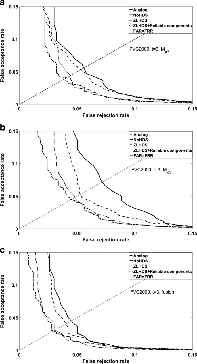
Performance result for several processing methods. FVC2000. Enrollment method E2 with t=3
Fig. 10 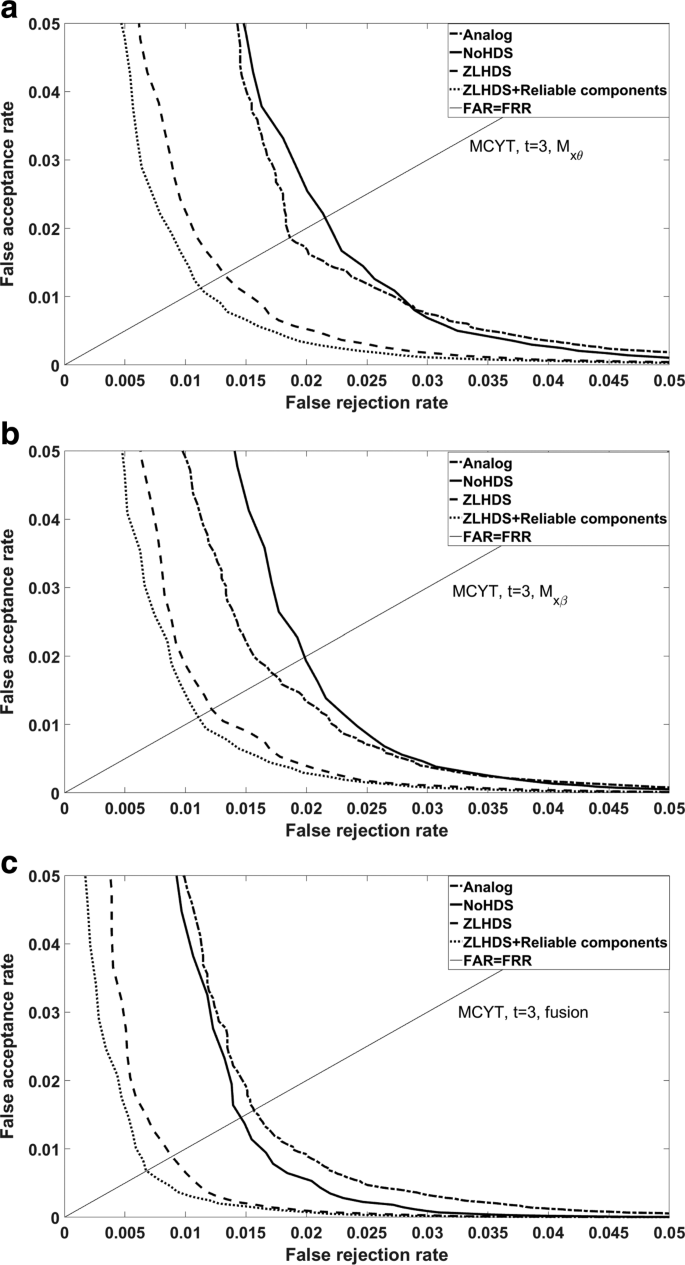
Performance result for several processing methods. MCYT. Enrollment method E2 with t=3
-
The E2 and E3 enrollment methods perform better than E1. Furthermore, performance increases with t. A typical example is shown in Fig. 11.
Fig. 11 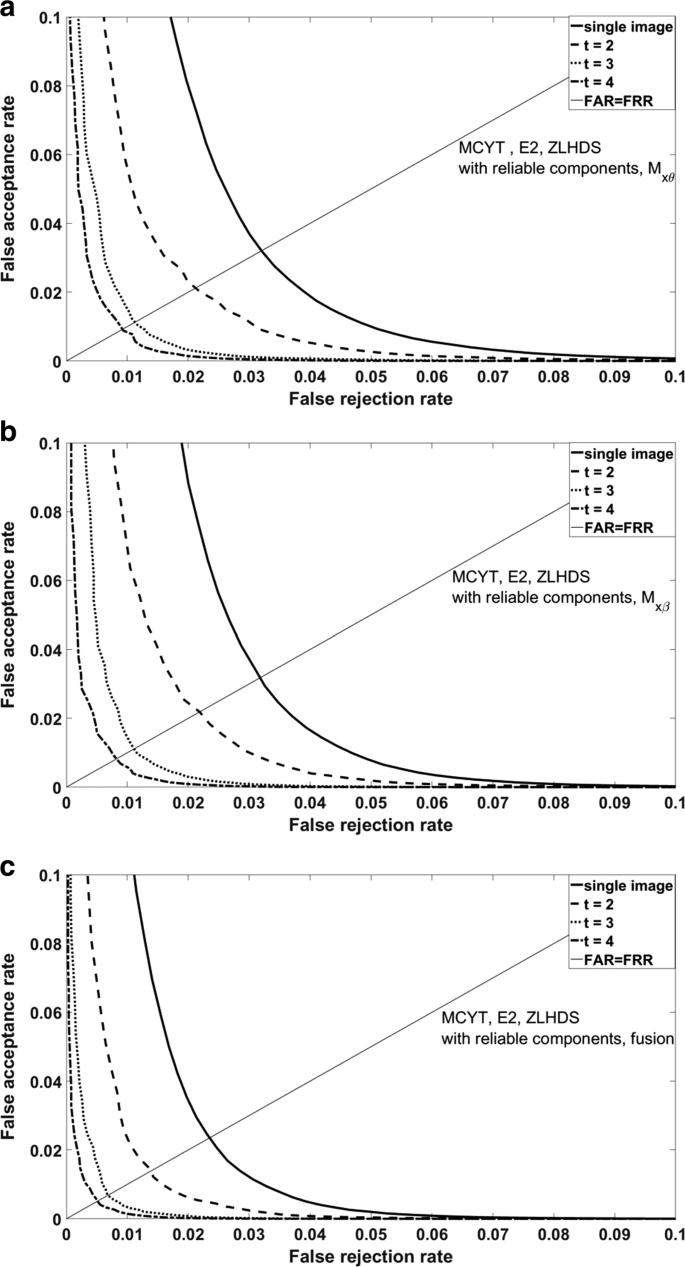
Performance effect of the number of images used for enrollment
-
The spectral functions \({\mathcal {M}}_{x\theta }\) and \({\mathcal {M}}_{x\beta }\) individually have roughly the same performance. Fusion yields a noticeable improvement. An example is shown in Fig. 12. (We implemented fusion in the analog domain as addition of the two similarity scores.)
Fig. 12 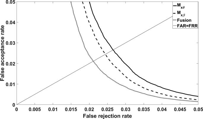
Performance of Mxθ and Mxβ individually, and of their fusion. MCYT database; enrollment method E1; analog domain
-
Tables 1, 2, 3, 4 and 5 show Equal Error Rates and Bit Error Rates. We see that enrollment methods E2 and E3 have similar performance, with E2 yielding a somewhat lower genuine-pair BER than E3.
Table 1 Equal error rates and bit error rates Table 2 EERs and BERs for the FVC2000 database Table 3 EERs and BERs for the FVC2002 database Table 4 EERs and BERs for the FVC2000 database Table 5 EERs and BERs for the MCYT database -
In Table 1 it may look strange that the EER in the rightmost column is sometimes lower than in the ‘analog’ column. We think this happens because there is no reliable component selection in the ‘analog’ procedure.
-
Ideally the impostor BER is 50%. In the tables we see that the impostor BER can get lower than 50% when the ZLHDS is used and the enrollment method is E2. On the other hand, it is always around 50% in the ‘No HDS’ case. This seems to contradict the Zero Leakage property of the helper data system. The ZLHDS is supposed not to leak, i.e. the helper data should not help impostors. However, the zero-leakage property is guaranteed to hold only if the variables are independent. In real-life data there are correlations between grid points and correlations between the real and imaginary part of a spectral function.


6.2 Error correction: Polar codes
The error rates in the genuine reconstructed \(\hat k\) are high, at least 0.21. In order to apply the Code Offset Method with a decent message size it is necessary to use a code that has a high rate even at small codeword length.
Consider the case of fusion of \({\mathcal {M}}_{x\theta }\) and \({\mathcal {M}}_{x\beta }\). The codeword length is 1280 bits (1024 if reliable component selection is performed). Suppose we need to distinguish between 220 users. Then the message length needs to be at least 20 bits, in spite of the high bit error rate. Furthermore, the security of the template protection is determined by the entropy of the data that is input into the hash function (see Fig. 2); it would be preferable to have at least 64 bits of entropy.
We constructed a number of Polar codes tuned to the signal-to-noise ratios of the individual grid points. The codes are designed to find a set of reliable channels, which are then assigned to the information bits. Each code yields a certain FAR (impostor string accidentally decoding correctly) and FRR (genuine reconstruction string failing to decode correctly), and hence can be represented as a point in an ROC plot. This is shown in Fig. 13. For the MCYT database we have constructed a Polar code with message length 25 at an EER around 1.2% (compared to 0.7% before error correction). For the FVC2000 database we have constructed a Polar code with message length 15 at ≈6% EER (compared to 3.3% EER before error correction). Note that the error correction is an indispensable part of the privacy protection and inevitably leads to a performance penalty. However, we see that the penalty is not that bad, especially for high-quality fingerprints.

FRR versus FAR achieved by Polar codes and random codebooks (average over three random codebooks). The \(\blacklozenge \) markers denote random codebook, and happen to coincide with the line connecting the Polar markers
We briefly comment on the entropy contained in the extracted ‘message’ strings. In Appendix A we present a method to compute the upper bound on the entropy of a random vector, in the case where the probability distribution obeys a number of symmetries. We use this method to get a rough estimate for the actual systems at hand. For the MCYT database and message length 25, the message bit means vary between 0.49 and 0.51, and the off-diagonal elements of the covariance matrix vary between −0.02 and 0.02. Applying the method of Appendix A with constant off-diagonal covariance 0.02 yields an upper bound of 24.3 bits of entropy. For FVC2000 with message length 15 bits, the bit means vary between 0.44 and 0.58, and the off-diagonal elements of the covariance matrix have magnitudes below 0.04. Applying the method of Appendix A with constant off-diagonal covariance 0.04 yields an upper bound of 14.1 bits of entropyFootnote 4. The actual entropies may be a lot lower than the estimates that we give here. Because of these low entropies, the data extracted from multiple fingers needs to be combined in order to achieve a reasonable security level of the hash. We do not see this as a drawback of our HDS; given that the EER for one finger is around 1%, which is impractical in real-life applications, it is necessary anyhow to combine multiple fingers.
6.3 Error correction: random codebooks
There is a large discrepancy between the message length of the Polar code (k≤25) and reported numbers for the information content of a fingerprint. According to Ratha et al. [30] the reproducible entropy of a fingerprint image with Z=35 robustly detectable minutiae should be more than 120 bits. Furthermore, the potential message size that can be carried in a 1024-bit string with a BER of 23% is 1024[1−h(0.23)]=227 bits. (And 122 bits at 30% BER.)
We experimented with random codebooks to see if we could extract more entropy from the data than with polar codes. At low code rates, a code based on random codewords can be practical to implement. Let the message size be ℓ, and the codeword size m. A random table needs to be stored of size 2ℓ·m bits, and the process of decoding consists of computing 2ℓ Hamming distances. We split the 1024 reliable bits into 4 groups of m=256 bits, for which we generated random codebooks, for various values of ℓ. The total message size is k=4ℓ and the total codeword size is n=4m. The results are shown in Fig. 13. In short: random codebooks give hardly any improvement over Polar codes.
7 Summary
We have built a HDS from a spectral function representation of fingerprint data, combined with a Zero Leakage quantisation scheme. It turns out that the performance degradation w.r.t. unprotected templates is caused mainly by the step that maps a list of minutiae to spectral functions. The step from unprotected spectral functions to HDS-protected spectral functions is almost ‘for free’ in the case of high-quality fingerprints.
The best results were obtained with the ‘superfinger’ enrollment method (E2, taking the average over multiple enrollment images in the spectral function domain), and with fusion of the \({\mathcal {M}}_{x\theta },{\mathcal {M}}_{x\beta }\) functions. The superfinger method performs slightly better than the E3 method and also has the advantage that it is not restricted to an odd number of enrollment captures.
For the high-quality MCYT database, our HDS achieves an EER around 1% and extracts an noise-robust 25-bit string that contains less than 24.3 bits of entropy. In practice multiple fingers need to be used in order to obtain an acceptable EER. This automatically increases the entropy of the hashed data. The entropy can be further increased by employing tricks like the Spammed Code Offset Method [31].
8 Conclusions
Any form of privacy protection (excepting perhaps homomorphic crypto) causes fingerprint matching degradation. Building a good template protection system is therefore an exercise in ‘damage control’: protect privacy while limiting the performance loss. We have pushed the two-dimensional spectral function approach to its limits, but even after the omission (in [20]) of the second invariant angle is corrected we still see that the transition from a minutia list to spectral functions destroys a lot of information. It remains a topic for future work to determine whether a higher-dimensional spectral function can retain more information while still yielding a practical template size. Given the experiences in [4] and the current paper, we expect that the ZLHDS privacy protection technique will do a good job there too, i.e. cause only little performance degradation, as long as the biometric data is of reasonable quality.
We see that Polar codes perform extremely well at the high BER caused by noisy biometrics. Polar codes have been used in a HDS before [23], but under somewhat different circumstances, namely a simple a priori known noise distribution. The results of Section 6.2 demonstrate the efficiency of Polar codes also in the case where the noise distribution is unknown and has to be estimated from the training data.
We briefly comment on the computational effort of our scheme in the verification phase. The number of (complex-valued) summation terms in the computation of a spectral function is \({Z\choose 2}N_{\text {grid}}\approx {35\choose 2}\cdot 20\cdot 16=1.9\cdot 10^{5}\). The reconstruction step of the first-stage ZLHDS has negligible cost compared to that. Successive Cancellation Decoding of Polar codes is lightweight, with complexity \({\mathcal {O}}(n\log n)\), n=1024. On a modern processor, computing a hash takes less than 100 clock cycles per input byte. Clearly the bottleneck is the computation of the spectral functions. We have observed that reducing the number of grid points from the current 20·16 causes severe degradation of the matching performance, while increasing the number of points does not yield much improvement.
As topics for future work we mention (i) testing the HDS on more databases; (ii) further optimisation of parameter choices such as the number of reliable components, and the number of minutiae used in the computation of the spectral functions; (iii) further tweaking of the Polar codes; (iv) other (spectral?) representations that cause less performance degradation while still allowing for a HDS to be constructed.
9 Appendix A
9.1 Entropy upper bound
Let X∈{0,1}n be a random variable with probability mass function px. Using the Lagrange multiplier technique it is readily ascertained that the maximum-entropy distribution for X, for given first and second moment, must be of the Gaussian form px∝ exp[−aTx−xTMx], where x is interpreted as a column vector, a is a vector and M is a matrix. In general the a and M are very complicated functions of the first moments \(m_{i}\overset {def}{=} \mathbb {E} x_{i}\) and the covariances \(c_{ij}\overset {def}{=} \mathbb {E} x_{i} x_{j} -m_{i} m_{j}\) (i≠j). The computations become more tractable if we impose permutation invariance on X as well as 0⇔1 symbol symmetry. Then we have \(p_{x}=N_{\beta }^{-1}\exp \left [\beta \left (|x|-\frac {n}{2}\right)^{2}\right ]\), where β is a parameter and the normalisation constant Nβ is defined as \(N_{\beta }=\sum _{w=0}^{n} {n \choose w}\exp \left [\beta \left (w-\frac {n}{2}\right)^{2}\right ]\). Furthermore the imposed symmetries yield \(m_{i}=\frac {1}{2}\) for all i, and constant covariance cij=c for i≠j. The relation between β and c is given by the 2nd moment constraint \(N_{\beta }^{-1}\sum _{w=0}^{n} \left (w-\frac {n}{2}\right)^{2} {n \choose w}\exp \left [\beta \left (w-\frac {n}{2}\right)^{2}\right ] =\frac {n}{4} +\left (n^{2}-n\right)c\). This equation has to be solved numerically for β. Then, with the numerical value of β, we can evaluate the entropy (in nats) as \(\mathbb {E} \ln \frac {1}{p_{x}}=\ln N_{\beta }-\beta \left [\frac {n}{4} +\left (n^{2}-n\right)c\right ]\).
Notes
Note that we often see correlations between the real and imaginary part. This has no influence on the ZLHDS.
We take the firstt images to show that the approach works. We are not trying to optimise the choice of images.
This is defined as a global property of the whole database. Our selection of reliable components does not reveal anything about an individual and hence preserves privacy. Note that [19] does reveal personalised reliable components and obtains better FA and FN error rates.
[12] extracts a 40-bit string.
Abbreviations
- BER:
-
Bit Error Rate
- COM:
-
Code Offset Method
- EER:
-
Equal Error Rate
- FAR:
-
False Acceptance Rate
- FRR:
-
False Rejection Rate
- HDS:
-
Helper Data System
- ROC:
-
Receiver Operating Characteristic
- SCD:
-
Successive Cancellation Decoder
- ZLHDS:
-
Zero Leakage Helper Data System
References
T. Matsumoto, H. Matsumoto, K. Yamada, S. Hoshino, in Proc. SPIE, Optical Security and Counterfeit Deterrence Techniques IV, vol. 4677. Impact of artificial “gummy” fingers on fingerprint systems, (2002), pp. 275–289.
D. Frumkin, A. Wasserstrom, A. Davidson, A. Grafit, Authentication of forensic DNA samples. FSI Genet.4(2), 95–103 (2010).
J. -P. Linnartz, P. Tuyls, in Audio- and Video-Based Biometric Person Authentication. New shielding functions to enhance privacy and prevent misuse of biometric templates (SpringerBerlin, 2003).
J de Groot, B Škorić, N de Vreede, J. P Linnartz, Quantization in Zero Leakage Helper Data Schemes. EURASIP J. Adv. Signal Process.2016:, 54 (2016).
T Stanko, F. N Andini, B Škorić, Optimized quantization in Zero Leakage Helper Data Systems. IEEE Trans. Inf. Forensics Secur.12(8), 1957–1966 (2017).
A. Juels, M. Wattenberg, in ACM Conference on Computer and Communications Security (CCS) 1999. A fuzzy commitment scheme, (1999), pp. 28–36.
Y. Dodis, R. Ostrovsky, L. Reyzin, A. Smith, Fuzzy Extractors: how to generate strong keys from biometrics and other noisy data. SIAM J. Comput.38(1), 97–139 (2008).
R. Canetti, B. Fuller, O. Paneth, L. Reyzin, A. Smith, in Eurocrypt 2016, Volume 9665. Reusable fuzzy extractors for low-entropy distributions, (2016), pp. 117–146.
J. Bringer, V. Despiegel, M. Favre, in Proc. SPIE 8029, Sensing Technologies for Global Health, Military Medicine, Disaster Response, and Environmental Monitoring; and Biometric Technology for Human Identification VIII. Adding localization information in a fingerprint binary feature vector representation, (2011), p. 80291O.
B. Topcu, Y. Z. Isik, H. Erdogan, in IEEE Conference on Computer Vision and Pattern Recognition (CVPR) Workshop. GMM-SVM fingerprint verification based on minutiae only (IEEE, 2016), pp. 155–160.
Z. Jin, M. H. Lim, A. B. J. Teoh, B. M. Goi, Y. H. Tay, Generating fixed-length representation from minutiae using kernel methods for fingerprint authentication. IEEE Trans. Syst. Man Cybern. Syst.46(10), 1415–1428 (2016).
P. Tuyls, A. H. M. Akkermans, T. A. M. Kevenaar, G. -J. Schrijen, A. M. Bazen, R. N. J. Veldhuis, in International Conference on Audio- and Video-Based Biometric Person Authentication (AVBPA). Practical biometric authentication with template protection (SpringerBerlin, 2005), pp. 436–446.
H Xu, R. N. J Veldhuis, A. M Bazen, T. A. M Kevenaar, A. H. M Akkermans, B Gokberk, Fingerprint verification using spectral minutiae representations. IEEE Trans. Inf. Forensics Secur.4(3), 397–409 (2009).
H. Xu, R. N. J. Veldhuis, in Int. Conf. on Biometrics: Theory, Applications and Systems (BTAS) 2009. Spectral minutiae representations of fingerprints enhanced by quality data (IEEE, 2009), pp. 1–5.
H. Xu, R. N. J. Veldhuis, in Image and Signal Processing (CISP) 2009. Spectral representations of fingerprint minutiae subsets (IEEE, 2009), pp. 1–5.
H. Xu, R. N. J. Veldhuis, in Computer Vision and Pattern Recognition Workshop. Complex spectral minutiae representation for fingerprint recognition (IEEE, 2010).
B. Topcu, H. Erdogan, C. Karabat, B. Yanıkoglu, in Int. Conf. of the Biometrics Special Interest Group (BIOSIG). Biohashing with fingerprint spectral minutiae (IEEE, 2013), pp. 254–265.
X. Shao, R. N. J. Veldhuis. IAPR Asian Conference on Pattern Recognition (IEEE, 2013), pp. 84–89.
K. Nandakumar, in Workshop on Information Forensics and Security (WIFS). A fingerprint cryptosystem based on minutiae phase spectrum (IEEE, 2010), pp. 1–6.
T. Stanko, B. Škorić, in IEEE Workshop on Information Forensics and Security (WIFS). Minutia-pair spectral representations for fingerprint template protection (IEEE, 2017).
F. Farooq, R. M. Bolle, T. -Y. Jea, N. Ratha, in IEEE Conference on Computer Vision and Pattern Recognition. Anonymous and revocable fingerprint recognition (IEEE, 2007), pp. 1–7.
Z. Jin, A. B. J. Teoh, T. S. Ong, C. Tee, in International Conference on Education Technology and Computer. Generating revocable fingerprint template using minutiae pair representation (IEEE, 2010), pp. 251–255.
B Chen, F. M. J Willems, Secret key generation over biased physical unclonable functions with polar codes. IEEE Internet Things J.6(1), 435–445 (2019).
T. M. Cover, J. A. Thomas, Elements of Information Theory (Wiley, Berlin, 2005).
E. Arıkan, Channel polarization: a method for constructing capacity-achieving codes for symmetric binary-input memoryless channels. IEEE Trans. Inf. Theory. 55(7), 3051–3073 (2009).
C. I. Watson, M. D. Garris, E. Tabassi, C. L. Wilson, R. M. McCabe, S. Janet, K. Ko, User’s guide to export controlled distribution of NIST biometric image software (2004). NISTIR 7391.
J. Ortega-Garcia, J. Fierrez-Aguilar, D. Simon, J. Gonzalez, M. Faundez, V. Espinosa, A. Satue, I. Hernaez, J. J. Igarza, C. Vivaracho, D. Escudero, Q. I. Moro, in Vision, Image and Signal Processing, Special Issue on Biometrics on the Internet, vol. 150. MCYT baseline corpus: A bimodal biometric database (IEEE, 2003), pp. 395–401.
D. Maltoni, D. Maio, A. K. Jain, S. Prabhakar, Handbook of Fingerprint Recognition, 2nd edn (Springer, London, 2009).
VeriFinger SDK. Available online. www.neurotechnology.com. Accessed 5 Aug 2019.
N. K. Ratha, J. H. Connell, R. M. Bolle, Enhancing security and privacy in biometrics-based authentication systems. IBM Syst. J.40:, 614–634 (2001).
B Škorić, N de Vreede, The Spammed Code Offset Method. IEEE Trans. Inf. Forensics Secur.9(5), 875–884 (2014).
Acknowledgements
We kindly thank the ATVS research group at Universidad Autonoma de Madrid for letting us use the MCYT database.
Funding
This study was partially funded by National Natural Science Foundation of China (NSFC, Chen, grant 61701155) and NWO (Stanko, grant 628.001.019).
Author information
Authors and Affiliations
Contributions
All authors contributed to this manuscript and fully endorse its content. All authors read and approved the final manuscript.
Corresponding author
Ethics declarations
Ethics approval and consent to participate
This article does not contain any studies with animals or humans performed by any of the authors.
Competing interests
The authors declare that they have no competing interests.
Additional information
Publisher’s Note
Springer Nature remains neutral with regard to jurisdictional claims in published maps and institutional affiliations.
Rights and permissions
Open Access This article is distributed under the terms of the Creative Commons Attribution 4.0 International License (http://creativecommons.org/licenses/by/4.0/), which permits unrestricted use, distribution, and reproduction in any medium, provided you give appropriate credit to the original author(s) and the source, provide a link to the Creative Commons license, and indicate if changes were made.
About this article

Cite this article
Stanko, T., Chen, B. & Škorić, B. Fingerprint template protection using minutia-pair spectral representations. EURASIP J. on Info. Security 2019, 12 (2019). https://doi.org/10.1186/s13635-019-0096-0
Received:
Accepted:
Published:
DOI: https://doi.org/10.1186/s13635-019-0096-0